Laminar Subnetworks of Response Suppression in Macaque Primary Visual Cortex

Abstract

Cortical inhibition plays an important role in information processing in the brain. However, the mechanisms by which inhibition and excitation are coordinated to generate functions in the six layers of the cortex remain unclear. Here, we measured laminar-specific responses to stimulus orientations in primary visual cortex (V1) of awake monkeys (male, Macaca mulatta). We distinguished inhibitory effects (suppression) from excitation, by taking advantage of the separability of excitation and inhibition in the orientation and time domains. We found two distinct types of suppression governing different layers. Fast suppression (FS) was strongest in input layers (4C and 6), and slow suppression (SS) was 3 times stronger in output layers (2/3 and 5). Interestingly, the two types of suppression were correlated with different functional properties measured with drifting gratings. FS was primarily correlated with orientation selectivity in input layers (r = -0.65, p < 10^-9), whereas SS was primarily correlated with surround suppression in output layers (r = 0.61, p < 10^-4). The earliest SS in layer 1 indicates the origin of cortical feedback for SS, in contrast to the feedforward/recurrent origin of FS. Our results reveal two V1 laminar subnetworks with different response suppression that may provide a general framework for laminar processing in other sensory cortices.SIGNIFICANCE STATEMENT This study sought to understand inhibitory effects (suppression) and their relationships with functional properties in the six different layers of the cortex. We found that the diversity of neural responses across layers in primary visual cortex (V1) could be fully explained by one excitatory and two suppressive components (fast and slow suppression). The distinct laminar distributions, origins, and functional roles of the two types of suppression provided a simplified representation of the differences between two V1 subnetworks (input network and output network). These results not only help to elucidate computational principles in macaque V1, but also provide a framework for general computation of cortical laminae in other sensory cortices.

Keywords: Macaque monkey; cortical layers; neural dynamics; primary visual cortex; suppression.

Figure 1.

Simultaneous recordings of multiple sites throughout V1 layers. A, Methods for laminar recording and reverse correlation. Left, Neural activity was recorded with U-Probe (Plexon, 24 channels, interchannel spacing 100 μm). The linear array was positioned vertically through the full depth of V1. Right, Demonstration of single trial and trial averages for MUA and LFP. Stimuli with different orientations were flashed for 20 ms in a random sequence. Shaded area represents the time window (−50 to 250 ms) for the triggered average. The neural activity of each channel was recorded with 2 ms resolution. Red represents sites within V1. B, Dynamics of orientation tuning of the MUA at three example sites at different cortical depths from the probe placement in A. Tuning curves were plotted every 10 ms, starting at 24 ms after stimulus onset and ending at 114 ms after stimulus onset. Red points represent the responses of the site to orientation at 0° (its preferred orientation). Blue points represent the responses of cells to orientation at 90° (orthogonal to preferred orientation). The tuning curves of each site were shifted, so that the preferred orientation was set to 0°. Dashed lines indicate the responses to a blank stimulus. C, Laminar pattern of MUA from 1 animal (DD). For each probe placement (P), the averaged responses of MUA to all orientations were calculated. Patterns in first column were averaged from all probe placements in this animal (N = 27). The relative cortical depth was determined by signatures of MUA and CSD (see Materials and Methods). Horizontal black dashed lines indicate the laminar boundaries. D, Similar to C, but for CSD of the same probe placements. Each CSD pattern was normalized by its SD.

Figure 2.

Population-averaged laminar pattern of orientation dynamics. A, Laminar pattern of orientation dynamics in a single probe placement. The snapshots were plotted starting at 0 ms; then every 6 ms was selected from 20 to 98 ms after stimulus onset. Each snapshot shows orientation tuning at all depths within V1. MUA response strength was coded by color. Each site's response was normalized by its maximum value. The length of the sliding window for averaging across depth is 0.1 (relative depth). Horizontal black dashed lines indicate the laminar boundaries. B, C, Similar to A, but averaged from multiple probe placements. B, Averaged from 1 animal (DD, MUA; N = 293). C, Averaged from another animal (DY, MUA; N = 114). D, Averaged from 70 SUAs of 2 animals (DD, N = 58; DY, N = 12). Color scale applies to A–D. E, An example for orientation dynamics of single unit (SUA) from experiment DD2-u035-003, channel #5. F, Orientation dynamics of MUA from the same recording site as in E. G, Orientation tuning of the example site (same as in E and F). The tuning averaged from 36 to 58 ms shown in E and F. Open circles represent SUA. Solid circles represent MUA. H, The comparison of orientation preferences between SUA and MUA (N = 58, FitR > 0.45). Circular correlation coefficient (r) is 0.72. I, The comparison of O/P ratio between SUA and MUA (N = 63, FitR > 0.1). Pearson's correlation coefficient (r) is 0.76. J, The comparison of orientation bandwidth between SUA and MUA (N = 52, FitR > 0.6). Pearson's correlation coefficient (r) is 0.86 (for details of the measurement of O/P ratio and bandwidth, see Materials and Methods).

Figure 3.

Three-component model for dynamic orientation tuning across V1 layers. Fitting population-averaged orientation dynamics within different layers used a three-component model. Different columns represent different aspects relative to model fitting. Different rows represent different layers. The second column represents raw normalized response (raw response). The third column represents the model fitted response pattern (fitted response). The first column represents the residual pattern (residual = raw response − fitted response). White numbers inset in the top left corner of each residual plot indicate the summed fitting error. The fourth to sixth columns represent three components (E, excitation; FS, fast suppression; SS, slow suppression) dissected from the dynamic response.

Figure 4.

Laminar pattern of neural dynamics can be fully explained by one excitatory and two suppressive mechanisms. The snapshots are plotted starting at 0 ms; then every 10 ms was selected from 20 to 150 ms after stimulus onset. Each snapshot shows orientation tuning of components at different cortical depths. The length of the sliding window is 0.1 (relative depth) in cortical space. A–C, The response at each depth was normalized by the corresponding peak value of the raw response at this depth. D–F, The strength at each depth was normalized by the corresponding peak value of excitation at this depth. Patterns of FS (E) and SS (F) were further normalized by the maximum values of FS and SS, respectively. Horizontal black dashed lines indicate the laminar boundaries. Sites with fitting error <0.13 were used (N = 395).

Figure 5.

Laminar distribution of the strength, latency, and orientation selectivity for excitatory and suppressive components. A, C, Laminar patterns of mean strength for FS and SS. Mean strength averaged from all orientations and normalized by corresponding maximum value of excitation (E). The length of sliding window is 0.1 (in relative depth) in cortical space. B, D, Laminar distribution of FS and SS Index (MUA; N = 395). The index was defined as the maximum value of mean strength. E, Latency of excitation (N = 395), FS (N = 346, FS Index > 0.12), and SS (N = 298, SS Index > 0.04). The latency was defined as the time at which each component first reached 2 × SDs of baseline fluctuations (−20 ms to 10 ms of raw dynamic response). F, Latency difference between FS and excitation (latency of FS minus latency of excitation) and SS and excitation (latency of SS minus latency of excitation). G, Laminar distribution of O/P ratio for excitation (N = 376, FitR > 0.1) and SS (N = 300, FitR > 0.1). H, Laminar distribution of bandwidth for excitation (N = 297, FitR > 0.6) and SS (N = 102, FitR > 0.6). Some depths are not shown in the plot of SS because the sliding windows did not include more than two sites.

Figure 6.

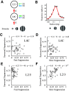
Correlation of two types of suppression with surround suppression. A, Schematic of the cascading relationship between the input layer (L4C) and output layer (L2/3). Stimuli were drifting sinusoidal gratings with different radius. Arrow thickness represents the strength of two types of suppression and excitation. B, Examples of individual tuning curves measured with drifting gratings of varying radius. Red curves indicate fits to the data (black dots) using the difference between two Naka–Rushton functions. Gray line indicates the spontaneous rate of firing. The example site was located in layer 2/3. C, D, Relationship between surround suppression and two types of suppression (C, FS; D, SS). Scatter plot for all sites of layer 4C. Strength of suppression defined as averaged strength from 0 to 200 ms. E, F, Similar to C, D but for all sites of layer 2/3.

Figure 7.

Correlation of three components with orientation selectivity. A, Schematic of the cascade relationship between input layer (L4C) and output layer (L2/3). Stimuli were drifting sinusoidal gratings with different orientations. Arrow thickness represents the strengths of suppression and excitation. B, C, Examples of individual tuning curves measured by drifting gratings of varying orientation. Red curves indicate fits to the data (black dots) using the von Mises function. Gray line indicates the spontaneous rate of firing. Example site in B located in layer 2/3. Example site in C located in layer 4C. D, Scatter plot of O/P ratio, measured with drifting gratings, against relative depth (N = 244). Horizontal black dashed lines indicate the laminar boundaries. E, Running average of O/P ratio at different cortical depth in D. The length of the sliding window for averaging across depth is 0.1 (relative depth) in cortical space. F–H, Relationship between O/P ratio calculated from tuning curves measured by drifting gratings and different mechanisms dissected from dynamic response (D, O/P ratio of excitation; E, FS; F, SS). Scatter plot for all sites of layer 4C. Strength of suppression defined as averaged strength from 0 to 200 ms. I–K, Similar to F–H, but for all sites of layer 2/3.

Figure 8.

Cascade effects of FS across layers. A, Scatter plot of FS of L4C and O/P ratio of L2/3 measured by drifting grating. For each MUA site of L2/3 (N = 76), we calculated the averaged integrated FS strength (from 0 to 200 ms) of all simultaneously recorded L4C sites. The Pearson's correlation coefficient (r) is −0.37. B, Population-averaged orientation tuning curves of L2/3 sites (N = 30 for each population). Black line indicates the average for the strong FS population in layer 4C (top 30). Gray line indicates the average for the weak FS population in layer 4C (last 30).

Figure 9.

RF mapping and preferred orientation estimation. A, RF mapping and preferred orientation estimation for an example probe placement. Left columns represent RFs as heat maps for sites through the depth of V1. The relative depth was labeled left to heat maps. Gray circle in each heat map represents the RF estimated by fitted Gaussian functions. Each RF map was normalized by its maximum value. Right columns represent orientation tunings of the same sites. Black curves indicate model (von Mises function) fits to the data (gray dots). Filled red dots represent sites' preferred orientations. B, RFs and orientation tunings of all sites recorded in the example probe placement in A. Only sites with well-fitted orientation tuning and RF are shown. Black dots represent RF centers of V1 sites. Left, The mean value of center distances among all pairs of RFs within V1 (MCD, 0.029) for the probe placement. Right, The mean value of absolute difference of orientation preferences among all pairs of tunings within V1 (MPD, 9.8) for the probe placement. C–J, Similar to A and B, but for another 4 probe placements. Color scale applies to all heat maps.

Figure 10.

Shifts of RF centers and orientation preferences. A, Distribution for MCDs from individual probe placement (N = 47 sessions). Black triangles represent mean value of the MCDs in all sessions. Gray dashed line indicates the threshold (0.08°). MCDs <0.08 visual angle occupy 83.0% (39 of 47) sessions. B, Distribution for mean value of absolute differences of orientation preferences (MPD) from individual probe placement (N = 47 sessions). Gray dashed line indicates the threshold (25°). MPDs <25°occupy 70.2% (33 of 47) sessions. C, Relationship between MCDs and MPDs for all valid probe placements. D, Shift of RF centers against relative depth. The shift of RF center of each recording site was defined as the center distance between the site's RF center and the RF center of L4C in the same probe placement (the site nearest to relative depth of 0.5). Each dotted line indicates 1 probe placement. Shaded areas represent regions in L2/3 or L5/6 (located at L2/3 and L5/6; range of relative depth, 0.05-0.25 for L2/3, 0.75-0.95 for L5/6) for further analysis in E and F. E, Scatter plot for shift of RF centers in L2/3 (relative to L4C in the same probe placement) against shift of RF center in L5/6 (relative to L4C in the same probe placement). Probe placements (N = 36) were included if L2/3, L4C, and L5/6 all have valid recording sites. F, Average shift of RF centers in L2/3 and L5/6 (both are relative to L4C; paired t test; n.s., not significant). G–I, Similar to D–F, but for shift of orientation preferences.

Figure 11.

Comparison of the shifts of orientation preferences between upper and lower layers relative to the input layers. Each column represents the comparison of shifts of orientation preferences between upper (L2/3) and lower (L5/6) layers relative to the input layers (L4C), with different selection criteria for perpendicular probe placements. The selection criteria are based on MCDs from individual probe placement. Probe placement with MCDs <0.04 deg for A and E, MCDs <0.05 deg for B and F, MCDs <0.06 deg for C and G, and MCDs <0.07 deg for D and H. A–D, Scatter plots for shift of orientation preferences in L2/3 against those in L5/6 (relative to orientation preferences in L4C). Probe placements with valid recording sites in both L2/3 and L5/6 were used. E–H, Average values of shifts of orientation preferences in L2/3 and average values of those L5/6. Nonsignificant values (paired t test; n.s., not significant).

Figure 12.

Summary of different types of suppression for laminar processing. A, Schematics of the results showing the distribution of FS and SS in V1. Green shading represents input layers (L4Cα, L4Cβ and L6) that receive geniculocortical input and have strong FS. Blue shading represents output layers (L2/3, L4B, and L5) which have strong SS. B, Schematics of the results regarding the functional properties of two types of suppression in orientation and spatial context processing. Excitation (red arrows) is the initial input of each layer. Red curve indicates tuning inherited from excitation. Black curve indicates the tuning modulated by suppression. The thickness of the arrows of FS (green arrows) and SS (blue arrows) represents the strength. The arrows around each tuning curve indicate the change in response magnitude caused by suppression.

References

1. Adesnik H, Bruns W, Taniguchi H, Huang ZJ, Scanziani M (2012) A neural circuit for spatial summation in visual cortex. Nature 490:226–231. 10.1038/nature11526 - DOI - PMC - PubMed
1. Adesnik H, Naka A (2018) Cracking the function of layers in the sensory cortex. Neuron 100:1028–1043. 10.1016/j.neuron.2018.10.032 - DOI - PMC - PubMed
1. Alitto HJ, Usrey WM (2008) Origin and dynamics of extraclassical suppression in the lateral geniculate nucleus of the macaque monkey. Neuron 57:135–146. 10.1016/j.neuron.2007.11.019 - DOI - PMC - PubMed
1. Allman J, Miezin F, McGuinness E (1985) Stimulus specific responses from beyond the classical receptive field: neurophysiological mechanisms for local-global comparisons in visual neurons. Annu Rev Neurosci 8:407–430. 10.1146/annurev.ne.08.030185.002203 - DOI - PubMed
1. Anderson JS, Carandini M, Ferster D (2000) Orientation tuning of input conductance, excitation, and inhibition in cat primary visual cortex. J Neurophysiol 84:909–926. 10.1152/jn.2000.84.2.909 - DOI - PubMed
Publication types
LinkOut - more resources