Siberian and temperate ecosystems shape Northern Hemisphere atmospheric CO2 seasonal amplification

Abstract

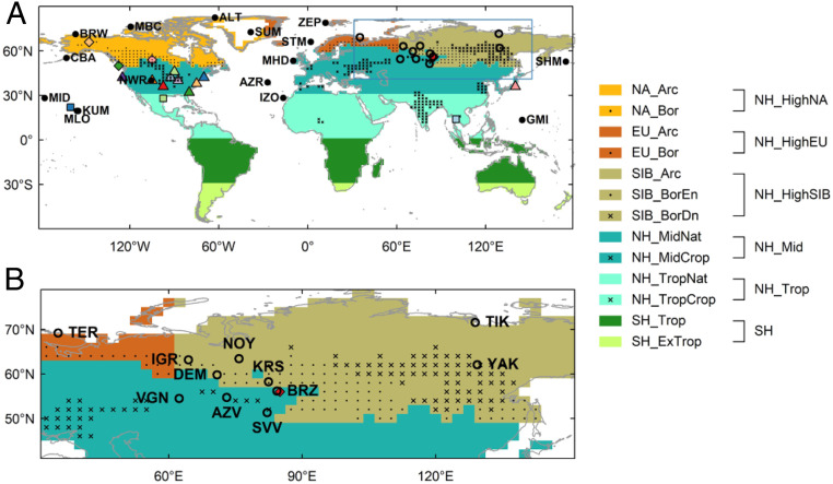
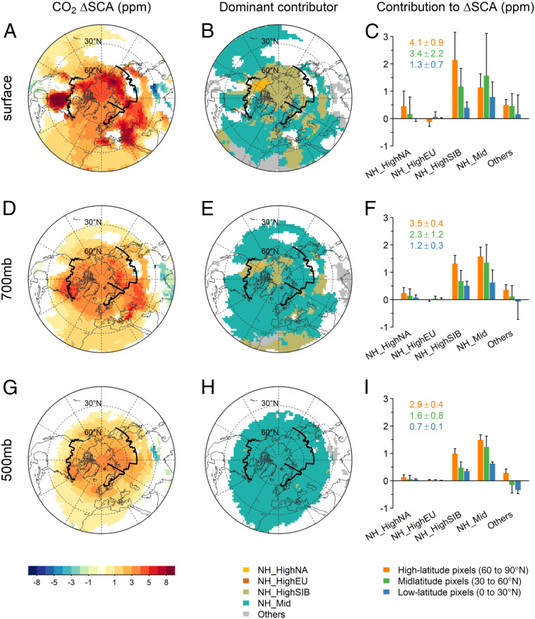
The amplitude of the atmospheric CO₂ seasonal cycle has increased by 30 to 50% in the Northern Hemisphere (NH) since the 1960s, suggesting widespread ecological changes in the northern extratropics. However, substantial uncertainty remains in the continental and regional drivers of this prominent amplitude increase. Here we present a quantitative regional attribution of CO₂ seasonal amplification over the past 4 decades, using a tagged atmospheric transport model prescribed with observationally constrained fluxes. We find that seasonal flux changes in Siberian and temperate ecosystems together shape the observed amplitude increases in the NH. At the surface of northern high latitudes, enhanced seasonal carbon exchange in Siberia is the dominant contributor (followed by temperate ecosystems). Arctic-boreal North America shows much smaller changes in flux seasonality and has only localized impacts. These continental contrasts, based on an atmospheric approach, corroborate heterogeneous vegetation greening and browning trends from field and remote-sensing observations, providing independent evidence for regionally divergent ecological responses and carbon dynamics to global change drivers. Over surface midlatitudes and throughout the midtroposphere, increased seasonal carbon exchange in temperate ecosystems is the dominant contributor to CO₂ amplification, albeit with considerable contributions from Siberia. Representing the mechanisms that control the high-latitude asymmetry in flux amplification found in this study should be an important goal for mechanistic land surface models moving forward.

Keywords: Arctic-boreal; amplification; carbon dioxide; global change; seasonal cycle.

Fig. 1.

(A) Map of tagged regions and northern surface stations used in this study. Filled circles indicate stations from NOAA's GGGRN assimilated in CAMSv17r1 CO₂ inversion, while open circles indicate Russian stations not assimilated. Colored symbols indicate grid cells where aircraft samples were assembled. (B) Close-up map from the blue box in A, marking Russian stations.

Fig. 2.

Evaluation of simulated versus observed (A) CO₂ SCA, (B) CO₂ ∆SCA, and (C) vertical difference in SCA between the altitude bins 0 to 1 km and 3 to 4 km. For A and B, filled (open) circles represent stations (not) assimilated in the CAMSv17r1 CO₂ inversion. The orange, green, and blue circles indicate high-latitude (60 to 90 °N), midlatitude (30 to 60 °N), and low-latitude (0 to 30 °N) stations. Dotted and solid lines represent the unit line and least squares regression line, respectively. The colored symbols in C correspond to those in Fig. 1A. Error bars denote ±1σ.

Fig. 3.

(A and C) Contribution of the six major tagged regions to site-level CO₂ SCA and ∆SCA in relation to (B and D) their NEE seasonal amplitudes (SCA_NEE) and changes (∆SCA_NEE). For A and C, the orange, green, and blue bars represent flux imprints from different tagged regions on x axis for northern high-latitude (60 to 90 °N; n = 7), midlatitude (30 to 60 °N; n = 5), and low-latitude (0 to 30 °N; n = 5) stations, respectively, with the numbers in the parentheses showing the mean SCA or ∆SCA averaged within station groups. Only the 16 stations from NOAA's GGGRN and the nonassimilated station Teriberka in Russia are included. For B and D, the gray and red bars represent the integrated and area-normalized SCA_NEE or ∆SCA_NEE for different tagged regions. Analyses were based on NEE from the CAMSv17r1 inversion for 1980 to 2017.

Fig. 4.

Spatial patterns of CO₂ ∆SCA and their dominant driving region in the NH. (A, D, and G) ∆SCA at the surface, 700 mb, and 500 mb calculated from model results with CAMSv17r1 for 1980 to 2017. Only pixels with significant trends (P < 0.05) are shaded. (B, E, and H) Maps of the dominant contributor to ∆SCA. For each pixel, this is the tagged region that imparts the largest ∆SCA. (C, F, and I) Zonal analyses of the regional contributions to ∆SCA. The orange, green, and blue bars represent flux imprints from different tagged regions on the x axis for northern high-latitude (60 to 90 °N), midlatitude (30 to 60 °N), and low-latitude (0 to 30 °N) pixels, respectively. The numbers on the top left show the mean ∆SCA averaged over each latitude band. Only pixels with significant positive trends (i.e., ∆SCA > 0, P < 0.05) were analyzed. The bold black lines delineate the three high-latitude tagged regions, i.e., NH_HighNA, NH_HighEU, and NH_HighSIB.

Fig. 5.

The trends in CO₂ SCA for aircraft profiles at four sites. (A–D) Comparison of simulated versus observed SCA trends for altitude bins between 1 and 8 km from aircraft profiles in Alaska (A), Massachusetts (B), Colorado (C), and Hawaii (D). Filled circles represent significant trends (P < 0.05), whereas open circles with pluses represent marginally significant trends (P < 0.1). Error bars show ±1σ. (E–H) Significance of the SCA trend as a function of data record length based on model results at each site (see details in Materials and Methods). The point of intersection between each curve and the horizontal dotted line represents the minimal data length required to achieve ≥50% detectability of a significant trend. For E, G, and H, the black lines represent the detectability curves for observations from the background stations Utqiagvik (Barrow; 11 m asl), Niwot Ridge (3,523 m asl), and Mauna Loa (3,399 m asl), which are in good agreement with model results at corresponding altitude levels.

References

1. Randerson J. T., Thompson M. V., Conway T. J., Fung I. Y., Field C. B., The contribution of terrestrial sources and sinks to trends in the seasonal cycle of atmospheric carbon dioxide. Global Biogeochem. Cycles 11, 535–560 (1997).
1. Keeling C. D., Chin J. F. S., Whorf T. P., Increased activity of northern vegetation inferred from atmospheric CO2 measurements. Nature 382, 146–149 (1996).
1. Graven H. D. et al. ., Enhanced seasonal exchange of CO2 by northern ecosystems since 1960. Science 341, 1085–1089 (2013). - PubMed
1. Randerson J. T., Field C. B., Fung I. Y., Tans P. P., Increases in early season ecosystem uptake explain recent changes in the seasonal cycle of atmospheric CO2 at high northern latitudes. Geophys. Res. Lett. 26, 2765–2768 (1999).
1. Barnes E. A., Parazoo N., Orbe C., Denning A. S., Isentropic transport and the seasonal cycle amplitude of CO2. J. Geophys. Res. 121, 8106–8124 (2016).
Publication types
LinkOut - more resources