Genome-Scale Imaging of the 3D Organization and Transcriptional Activity of Chromatin

Abstract

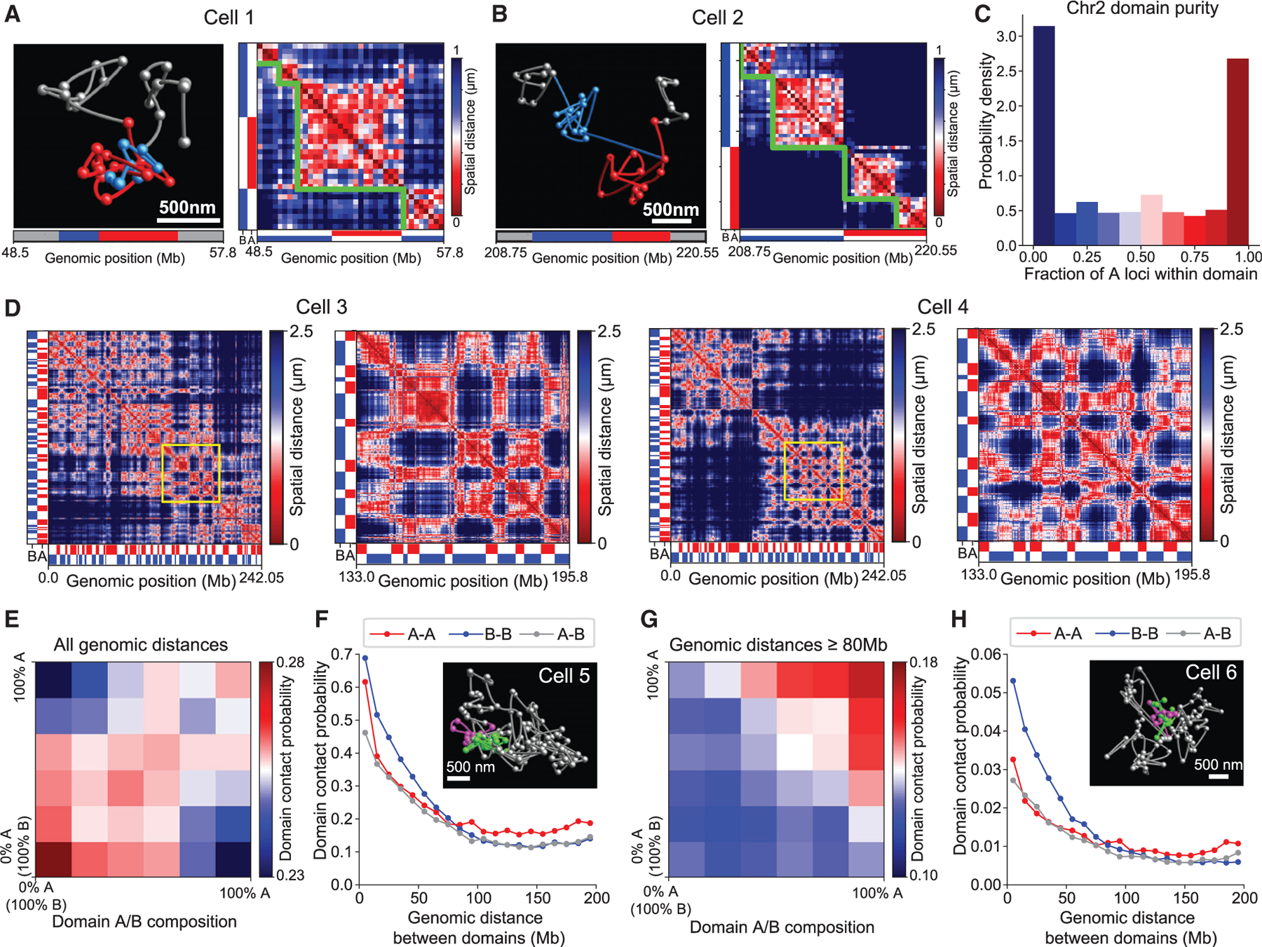
The 3D organization of chromatin regulates many genome functions. Our understanding of 3D genome organization requires tools to directly visualize chromatin conformation in its native context. Here we report an imaging technology for visualizing chromatin organization across multiple scales in single cells with high genomic throughput. First we demonstrate multiplexed imaging of hundreds of genomic loci by sequential hybridization, which allows high-resolution conformation tracing of whole chromosomes. Next we report a multiplexed error-robust fluorescence in situ hybridization (MERFISH)-based method for genome-scale chromatin tracing and demonstrate simultaneous imaging of more than 1,000 genomic loci and nascent transcripts of more than 1,000 genes together with landmark nuclear structures. Using this technology, we characterize chromatin domains, compartments, and trans-chromosomal interactions and their relationship to transcription in single cells. We envision broad application of this high-throughput, multi-scale, and multi-modal imaging technology, which provides an integrated view of chromatin organization in its native structural and functional context.

Keywords: 3D genome organization; MERFISH; chromosome compartments; chromosome conformation; genome-scale imaging; multiplexed FISH; nuclear lamina; nuclear speckles; topologically associated domains; trans-chromosomal interaction.

Figure 1.. High-Resolution Whole-Chromosome Tracing by Sequential Hybridization and Characterization of Chromatin Domains in Single Cells

(A) Schematics of the multi-scale chromatin tracing platform. Left: schematic of chromosome tracing by sequential hybridization and imaging. A single chromatin locus is imaged in each color channel per imaging round. After many rounds of imaging, a 3D chromatin trace can be generated for each copy of the targeted chromosome. Right: schematic of genome-scale imaging by DNA-MERFISH. Multiple loci are imaged and resolved in each round, and the identity of each locus can be derived from a barcode based on the combination of rounds in which the locus is detected. This approach significantly reduces the number of rounds required to image the same number of loci compared with the sequential imaging approach. (B) 3D structural rendering and spatial distance matrices of the two copies of Chr21 in a single IMR90 cell imaged using the sequential hybridization approach. Left: the two copies of Chr21 in a single cell (red and green) are overlaid on a DAPI image of the nucleus (blue). Top right: 3D rendering of all detected chromatin loci (colored spheres) in the two Chr21 copies, color-coded according to their genomic coordinates along the chromosome (color index shown on the right). Flexible lines connect adjacent chromatin loci. Bottom right: pairwise spatial distance matrices corresponding to the chromosome copies displayed above (genomic regions without proper reference genomes or containing highly repetitive sequences are not imaged). The genomic positions of the start of the first targeted locus and the end of the last targeted locus are indicated. If a targetted locus was not detected, the matrix elements representing its spatial distances to other loci are shown in black. (C) Ensemble proximity frequency matrix of Chr21 and preferential positioning of single-cell domain boundaries at CTCF/cohesin-binding sites. Top: proximity frequency matrix for Chr21. Each matrix element is defined as the frequency with which the measured distance between that pair of loci is shorter than a cutoff distance of 500 nm. Center: magnified version of the proximity frequency matrix for a 10-Mb portion of Chr21. Bottom: the probability of single-cell domain boundary formation at each of the imaged 50-kb segments. Orange and yellow triangles show CTCF and RAD21 (a subunit of cohesin complex) chromatin immunoprecipitation sequencing (ChIP-seq) peaks (Dunham et al., 2012), respectively. (D) Average probability of domain boundary formation in single cells as a function of the genomic distance to CTCF/Rad21-binding sites (sites bound by both proteins, yellow) or to ensemble TAD boundaries (gray). (E) Example of two single-cell chromatin domains with identical genomic coordinates occupying large (top) or small (bottom) volumes in physical space. Left: 3D rendering of the chromatin domains, with green balls representing imaged genomic loci within the domain. Grey spots represent imaged loci in the rest of the chromosome. Right: pairwise distance matrix for the chromatin domain shown on the left (marked with green lines) with flanking regions. (F) Example of two pairs of chromatin domains with high (top) and low (bottom) insulation scores. Left: 3D rendering of the chromatin domains. The neighboring domains are shown in green and magenta. Right: pairwise distance matrix for the chromatin domains shown on the left, with rendered domains marked in corresponding colors. (G) Two examples of long-range contact between chromatin domains. Left: 3D rendering of the chromatin domains, with different colors representing different domains. Right: pairwise distance matrix for the chromatin domains, with rendered domains marked in corresponding colors. The gray space in the bottom right panel indicates a gap in genomic distance of 22.85 Mb. (H) Example of chromatin domains (green) flanked by CTCF binding sites (red), showing small (top) and large (bottom) distances between the CTCF sites. Left: 3D rendering of the chromatin domain. Right: pairwise distance matrix for the chromatin domain, with domain and border CTCF marked correspondingly. (I) Distribution of genomic sizes of domains in Chr21 in single cells (green). Shown in the black outline is the distribution of genomic sizes of domains in Chr21 derived from data simulating a localization error of 100 nm. In this simulation, the positions of the imaged loci are perturbed with a 3D Gaussian noise with a standard deviation of 100 nm, similar to our measurement error. (J) Distribution of physical sizes, as defined by the radii of gyration, of domains in Chr21 in single cells (green). Shown in the black outline is the distribution of physical sizes of domains in Chr21, derived from data simulating a localization error of 100 nm, as in (I). (K) Median radius of gyration as a function of genomic size for chromatin domains with boundary loci containing interacting CTCF/Rad21 sites (orange) and with neither boundary locus containing CTCF/Rad21 sites (gray). Interacting CTCF/Rad21 sites are defined as those that formed loops in Hi-C maps (Rao et al., 2014). Error bars indicate 95% confidence intervals derived by resampling. (L) Distribution of insulation scores between neighboring domains with domain boundaries occurring at CTCF/Rad21-binding sites (orange) and non-CTCF/Rad21-binding sites (gray). (M) Median of normalized distance between the boundary loci of domains as a function of genomic size for chromatin domains with boundary loci containing interacting CTCF/Rad21 sites (orange), as defined in (K), and with neither boundary locus containing CTCF/Rad21 sites (gray). The normalized distance between boundary loci is defined as the distance between the domain’s boundary loci divided by the median distance between the same type of locus pairs separated by the same genomic distance but lying in the interior of a single domain. Error bars indicate 95% confidence intervals derived by resampling.

Figure 2.. Compartment Structure in Single Chromosomes and Relationship between Transcription Activity and Local Chromatin Content

(A) Pearson correlation matrix for genomic distance-normalized proximity frequencies of Chr21, derived from our imaging data. Two loci are considered in proximity when their distance is smaller than a cutoff distance of 500 nm. Two bars at the bottom shows the A/B calling derived from the proximity frequency matrix (shown in red and blue for A and B compartments, respectively) and the G-banding (National Center for Biotechnology Information, 2020; shown in grayscale) of each genomic locus in the chromosome. (B) 3D rendering of individual copies of Chr21, with A and B loci shown as red and blue balls, respectively. The bar at the bottom shows the A/B calling of each genomic locus in the chromosome, derived from proximity frequency matrix. (C) Distribution of the A/B segregation score for individual copies of Chr21, shown in orange. To calculate the A/B segregation score, we defined an A (or B) dense volume for each chromosome copy by thresholding the local A (or B) density so that two-thirds of A (or B) loci with the highest A (or B) density score were contained within the volume (note that the A and B dense volumes can overlap). We further defined the purity of loci in the A (or B) dense volume of the chromosome copy as the fraction of all loci within the volume being A (or B) loci and defined the A/B segregation score of the chromosome copy as the mean purity of the A and B volumes. The gray histogram represents the distribution of A/B segregation scores for a randomization control, where the boundaries between contiguous A and B regions are shifted along the genomic sequence by a random amount for each imaged chromosome copy (in a cyclic fashion after joining the imaged chromosome ends), which keeps the number of A/B boundaries and the sizes of A and B regions largely unchanged, except for the regions at the chromosome ends. (D) Pearson correlation matrix for genomic distance-normalized proximity frequencies for the p and q arms of Chr2 and corresponding A/B calling and G-banding as in (A). (E) 3D renderings of individual copies of Chr2 as in (B). (F) Distribution of A/B segregation scores for Chr2 in single cells as in (C). (G) 3D rendering of a single copy of Chr21 shown together with transcriptional bursts of the measured genes. Chromatin is rendered in red (A loci) and blue (B loci) as in (B). Yellow balls represent the locations of all detected nascent RNA foci in this chromosome. (H) Change (measured in log difference) in the A/B density ratios at the transcription start sites (TSSs) of the imaged genes between actively firing and non-firing states. For each gene, we compute the median A/B density ratio at its TSS in chromosomes where the gene is firing and in chromosomes where it is not firing. The log difference of these median values for the ~80 genes imaged on Chr21 is rank ordered according to the magnitude of change in their median A/B density ratios. Log difference stands for the difference in log values. (I) Change (measured in log difference) in the firing rates of imaged genes as the environment of the gene’s TSS is changed from low (bottom quartile) to high (top quartile) A/B density ratios. The log difference in firing rate for the ~80 genes imaged on Chr21 is rank ordered according to the magnitude of firing rate change.

Figure 3.. Dependence of Domain-Domain Interaction on A/B Composition and Genomic Distances

(A) Left: 3D rendering of a “mixed” chromatin domain containing A and B loci (displayed as red and blue balls, respectively), flanked by pure domains comprised of only B loci (displayed as gray balls) in a single copy of Chr2. Right: pairwise distance matrix for the region displayed on the left. The red and blue bars on the bottom and left display the A (red) and B (blue) calling of loci, and the green outline highlights the boundaries of the chromatin domains. (B) Same as in (A) but for two pure domains, one comprised entirely of A loci and one of B loci, instead of a mixed domain. (C) Distribution of the fraction of loci being A loci in single-cell chromatin domains in Chr2. (D) Single-cell spatial distance matrices of two example copies of Chr2. The first and third panels show the matrix for two whole chromosomes, whereas the second and last panels show a magnified matrix for the region highlighted in yellow in the first and third panels, respectively. The side bars show the A (red)/B (blue) compartment calling. (E) Domain contact probabilities for domains of different A/B compositions in Chr2. The x and y axes represent the fraction of loci within a domain being A loci (0% corresponds to pure B domain and 100% corresponds to pure A domain). Two domains are defined to be in contact when their insulation score is less than 2. See STAR Methods for calculation of the insulation score. (F) Domain contact probability between pure A domains (A-A), between pure B domains (B-B), and between pure A and pure B domains (A-B) in Chr2, plotted asa function of the genomic distance between the two domains. The inset shows a 3D rendering of an example pair of domains displaying long-range interaction with an insulation score of ~2. The two interacting domains are displayed in green and magenta, whereas the chromatin in between is displayed in gray. (G) Same as (E) but for domain pairs with genomic distances larger than 80 Mb. (H) Same as (F), but restricted to domain pairs with a high degree of intermixing (as defined by a low insulation score of less than 1). The inset shows a 3D rendering of an example pair of domains displaying long-range interaction with a high degree of intermixing (insulation score being ~1).

Figure 4.. Genome-Scale Chromatin Imaging by DNA-MERFISH

(A) Imaging scheme of DNA-MERFISH. The targeted genomic loci are assigned error-robust barcodes; e.g., a subset of 100-bit HW2 binary barcodes. The barcodes are imprinted onto the genomic loci with encoding oligonucleotide probes that recognize the loci and associate two distinct readout sequences with each locus, corresponding to the two bits that read 1 in the barcode assigned to the locus. Each locus is labeled by a total of ~400 encoding probes, but only 4 are shown. Fluorescent readout probes complementary to the readout sequences are sequentially added and imaged, allowing the bits that read 1 at each locus (and, hence, the barcode identity of that locus) to be determined. (B) Representative images from multiple imaging rounds in the nucleus of a single cell. The fluorescent signal of the chromatin loci from readout probes is shown in yellow, whereas the DAPI signal, used as a nuclear marker, is shown in blue. (C) Magnified images of a small region (white box in B) centered around one chromatin locus across all imaging rounds, with two bits (1 and 13) on. (D) A 3D rendering of all detected chromatin loci (colored spheres) in a single IMR-90 cell, color-coded according to the chromosomes to which they belong (color index for chromosomes shown below the image). Adjacent loci in genomic sequence are connected by a flexible line. 1,041 genomic loci are targeted. (E) Chromatin loci of the same cell as in (D) but with two homologs of the indicated chromosomes shown in color and all other loci shown in gray. (F) Median distance matrix computed from ~5,400 single cells. For each pair of loci, the median of observed 3D spatial distances between the loci across all cells is presented. (G) Example images showing the positions of multiple chromosomes territories in single cells. Chromosomes are color-coded as indicated, and shaded areas represent the convex hull surrounding all imaged loci. Only one homolog is shown per chromosome for clarity. (H) Spatial distance matrices for the cells shown in (G). Chromosome order is as noted beneath the matrices, with the two homologs of each chromosome shown separately.

Figure 5.. Enrichment of Active-Active Chromatin Interactions in trans-Chromosomal Interactions

(A) Normalized trans-chromosomal proximity frequency matrix. The normalized proximity frequency between each trans-chromosomal locus pair is shown, with pairs of loci considered to be in proximity when their distancesare smaller than a cutoff distance of 500 nm. The loci are reordered so that compartment A loci appear first, followed by compartment B loci. Each entry in the matrix shows the proximity frequency between a trans-chromosomal locus pair normalized by the median proximity frequency of all locus pairs originating from the same pair of chromosomes to account for varying basal levels of interaction between pairs of chromosomes. (B) Distributions of normalized trans-chromosomal proximity frequencies for pairs of A loci (A-A, red), pairs of B loci (B-B, blue), and pairs comprised of one A and one B locus (A-B, gray), derived from the matrix shown in (A). Distributions are represented in the top panel as histograms and in the bottom panel as boxplots, showing the median (center lines), 25^th–75^th percentiles (boxes) and 5^th–95^th percentiles (whiskers). (C) The proximity frequency between pairs of cis chromatin loci within the same chromosomes as a function of their genomic distance, for pairs of loci separated by the same genomic distance across all chromosomes. The proximity frequencies are calculated across all chromosomes for pairs of loci separated by the same genome distance and are shown for pairs of A loci (A-A, red), pairs of B loci (B-B, blue), and mixed pairs of A and B loci (A-B, gray). (D) Distributions of A and B loci in two single cells. The left panels show the locations of all detected loci within a singlez plane ina nucleus, with A loci shown in red and B loci shown in blue. In the right panels, the color of each locus represents the ratio of the local densities of trans-chromosomal A and B loci (i.e., the trans A/B density ratio), in accordance with the color scale bar shown on the right. (E) Distributions of the median trans A/B density ratio for imaged genomic loci. For each locus, the median trans A/B density ratio across all cells was determined, and the trans A/B density ratio distribution for A loci is shown in red and for B loci in blue. The dark gray histogram represents a randomization control where A and B compartment identity is shuffled randomly while keeping the total numbers of A loci and B loci unchanged. This histogram is cropped by the y-axis range, which is set to allow a clearer visualization of the histograms for the A and B loci.

Figure 6.. Multi-modal Genome-Scale Imaging of Chromatin and Transcription Activity in the Context of Nuclear Structures

(A) Top: illustration of the multi-modal imaging scheme combining chromatin (left panel), nascent RNA (center panel), and nuclear body (right panel) imaging. Approximately 1,000 genomic loci, nascent RNA transcripts of ~1,100 genes in the targeted loci, and two types of nuclear bodies (nuclear speckles and nucleoli) are imaged. Bottom: representative raw images for each imaging modality: chromatin loci across multiple imaging rounds (left), nascent RNA transcripts across multiple imaging rounds (center), and nuclear bodies (right; yellow, nuclear speckles imaged using an anti-SC35 antibody; blue, nucleoli imaged using an antifibrillarin antibody). (B) 3D rendering of chromatin loci, transcriptional foci, and nuclear bodies in a single cell. Left: all detected chromatin loci, color-coded by chromosome (based on the chromosome index shown below). Center: all detected foci of nascent transcripts shown as colored spheres, with colors indicating the identities of the imaged genes and sphere size representing transcription burst size. Chromatin loci are shown in gray. Right: volume-filling representations of detected nuclear bodies. Nucleoli are shown in blue and nuclear speckles in yellow. The nuclear lamina is identified as the surface of the convex hull surrounding all detected chromatin loci (shaded gray area). (C and D) Distributions of transcription burst frequencies (C) and burst sizes (D) for genes residing in the imaged A loci (red) and B loci (blue). (E and F) Distributions of association rates for A loci (red) and B loci (blue) with the nuclear lamina (E) and nuclear speckles (F). A chromatin locus is considered associated with a nuclear body when the distance of the locus to that body is less than 250 nm. (G and H) Scatterplots of the median trans A/B density ratio for each imaged genomic locus as a function of the frequency with which the locus is associated with the nuclear lamina (G; Pearson correlation coefficient = −0.87) and nuclear speckles (H; Pearson correlation coefficient = 0.66). (I) Association frequency with nucleoli for all imaged genomic loci, ordered by genomic position. Black vertical lines indicate the locations of centromeres, and red brackets highlight chromosomes containing ribosome-encoding genes (rDNAs). (J) Correlation of transcription with nuclear structure association. Circles represent the fold change in transcriptional burst frequency for individual genomic loci when comparing the populations of cells in which the locus is lamina associated versus non-lamina-associated (left) and speckle-associated versus non-speckle associated (right). The dotted red line indicates no change, and the solid red lines represent the median fold change in each case.

Figure 7.. Correlation between Transcriptional Activity and Local Enrichment of trans-Chromosomal Active Chromatin

(A) Single-cell images of chromatin loci and transcriptional activities. Left: locations of all imaged A (red) and B (blue) loci in a single z plane from a nucleus. Center: trans A/B density ratios for the same loci, color-coded based on the color scale bar. Right: same as the center panel but with detected transcriptional bursts displayed as green circles. (B) Change (measured in log difference) in the trans A/B density ratios for each imaged locus between actively firing and non-firing states. For each genomic locus containing at least one imaged gene, the median trans A/B density ratio was calculated for cells in which the genomic locus was actively transcribing and for cells in which it was not transcribing (silent). The log difference of these median values for each imaged locus was rank ordered according to the magnitude of change of these values. (C) Change (measured in log difference) in the firing rates of the imaged gene-harboring loci between cells in which the trans A/B density ratio at the locus is low (bottom quartile) and cells in which this value is high (top quartile). The log-difference in firing rate for the imaged loci was rank-ordered according to the magnitude of the firing rate change. (D) Change (measured in log difference) in trans A/B density ratios between transcribed and silent states for the imaged gene-containing loci, conditioned on their nuclear body association status. For each genomic locus, we computed the fold change in the trans A/B density ratio between transcribed and silent states of the locus, considering, from left to right, respectively, all cells (black circles), only cells in which the locus was associated with a nuclear speckle (yellow circles), only cells in which the locus was associated with the lamina (blue circles), and only cells in which the locus was not associated with a nuclear speckle or the lamina (hollow circles). The median trans A/B density ratio in each state (transcribed or silent) was determined for each locus, and each association condition and the log2 of the fold change between the two states are shown. The dotted red line represents no change, and the solid red lines represent the median log difference across all loci in each case. Some outliers were omitted to allow clearer visualization of the median log difference (14, 54, and 3 outlier loci for speckle-associated data, lamina-associated data, and not lamina-associated and not-speckle-associated data, respectively).

References

1. Abramo K, Valton A-L, Venev SV, Ozadam H, Fox AN, and Dekker J (2019). A chromosome folding intermediate at the condensin-to-cohesin transition during telophase. Nat. Cell Biol 21, 1393–1402. - PMC - PubMed
1. Beagrie RA, Scialdone A, Schueler M, Kraemer DCA, Chotalia M, Xie SQ, Barbieri M, de Santiago I, Lavitas L-M, Branco MR, et al. (2017). Complex multi-enhancer contacts captured by genome architecture mapping. Nature 543, 519–524. - PMC - PubMed
1. Bickmore WA (2013). The spatial organization of the human genome. Annu. Rev. Genomics Hum. Genet 14, 67–84. - PubMed
1. Bintu B, Mateo LJ, Su J, Sinnott-Armstrong NA, Parker M, Kinrot S, Yamaya K, Boettiger AN, and Zhuang X (2018). Super-resolution chromatin tracing reveals domains and cooperative interactions in single cells. Science 362, eaau1783. - PMC - PubMed
1. Bolzer A, Kreth G, Solovei I, Koehler D, Saracoglu K, Fauth C, Müller S, Eils R, Cremer C, Speicher MR, and Cremer T (2005). Three-dimensional maps of all chromosomes in human male fibroblast nuclei and prometaphase rosettes. PLoS Biol 3, e157. - PMC - PubMed
Publication types