Arctic tidal current atlas

Abstract

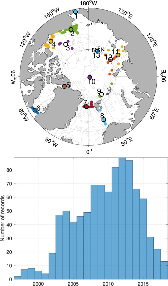
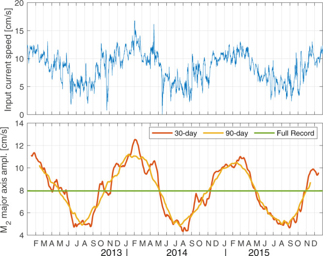
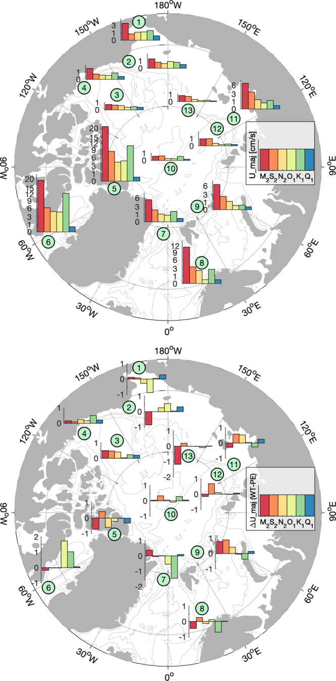
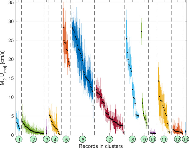
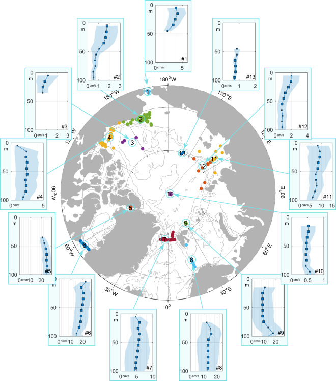
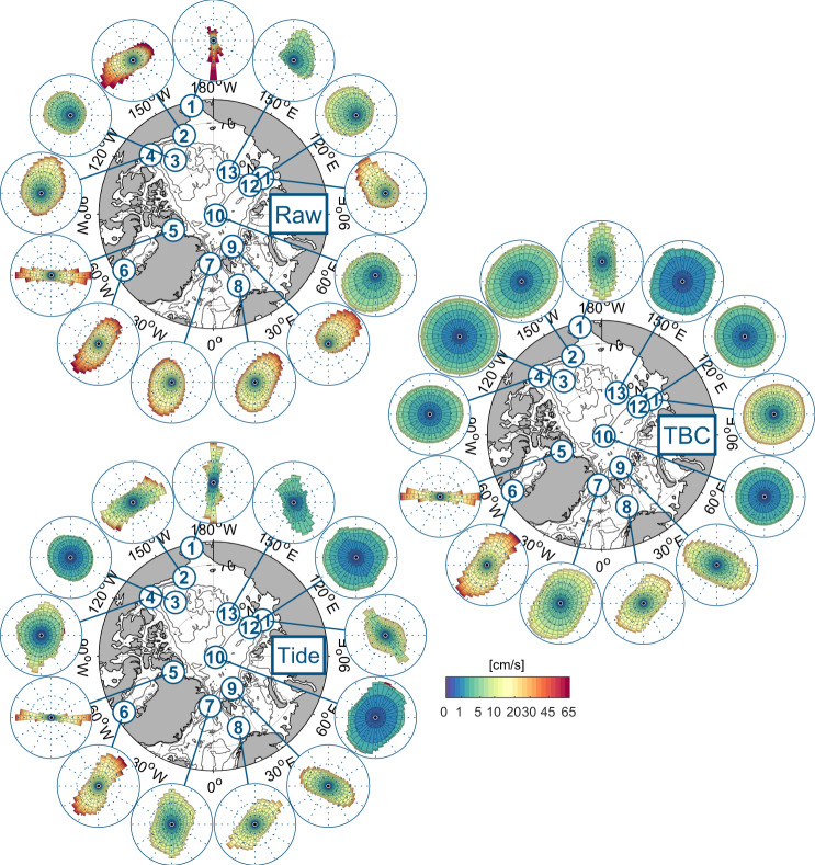
Tidal and wind-driven near-inertial currents play a vital role in the changing Arctic climate and the marine ecosystems. We compiled 429 available moored current observations taken over the last two decades throughout the Arctic to assemble a pan-Arctic atlas of tidal band currents. The atlas contains different tidal current products designed for the analysis of tidal parameters from monthly to inter-annual time scales. On shorter time scales, wind-driven inertial currents cannot be analytically separated from semidiurnal tidal constituents. Thus, we include 10-30 h band-pass filtered currents, which include all semidiurnal and diurnal tidal constituents as well as wind-driven inertial currents for the analysis of high-frequency variability of ocean dynamics. This allows for a wide range of possible uses, including local case studies of baroclinic tidal currents, assessment of long-term trends in tidal band kinetic energy and Arctic-wide validation of ocean circulation models. This atlas may also be a valuable tool for resource management and industrial applications such as fisheries, navigation and offshore construction.

Fig. 1

Spatial and temporal distribution of current velocity records contained in the atlas. Top: Map showing locations of the records (coloured dots). Colours indicate grouping utilized for visualizations. Black circles show the centroid location and number of each cluster. Bottom: Histogram of record distribution over time.

Fig. 2

Tidal analysis using different window lengths performed on an artificial time series. The time series is constructed to resemble realistic conditions found at the eastern Eurasian continental slope (see Baumann et al.) and consists of a complex harmonic oscillation at M₂ frequency with an amplitude of 8 cm/s. The amplitude undergoes a seasonal cycle represented by a cosine function with 365.25-day period and amplitude of 3 cm/s. To this, we added inertial oscillations (average amplitude ~2 cm/s) simulated from a slab-model with 50-m SML (see for details). The 30-day and 90-day analyses predominantly follow the seasonal cycle, but noise has a substantial impact on the 30-day analysis. Some minor distortions of the seasonal signal are also visible for the 90-day analysis. The full-record analysis produces a single set of tidal ellipse parameters with the major axis amplitude almost exactly matching the input.

Fig. 3

Major axis amplitudes of tidal constituents (U_maj) from full-record analysis and their comparison to a barotropic tidal model. (top) Amplitudes are averaged vertically and over all records within each cluster. (bottom) Difference of U_maj for tidal constituents from full-record analysis and barotropic model output. Model data stems from Padman and Erofeeva.

Fig. 4

Spatio-temporal variability of tidal currents, illustrated by the range of M₂ U_maj (from 30-day (light shading) and 90-day (solid colour) analysis, at 50 m depth) for each record in each cluster. The records within each cluster are sorted by average U_maj (black dots). For readability, horizontal plotting space was stretched for clusters with a smaller number of records (clusters #5 and #7-#13).

Fig. 5

Cluster-average profiles of M₂ major axis amplitudes from 90-day analysis over the top 100 m. Averages were taken over 10 m bins with squares in the profiles showing the center of the bins and the sizes reflect the relative number of measurements in that bin. Shading denotes ±1 standard deviation. The (linear) x-axis scales are different in each plot, but the vertical grid lines are always spaced by 2 cm/s.

Fig. 6

Regional current roses for observed raw currents (top), tidal band currents (TBC, right) and tidal prediction from full-record analysis (bottom). The roses are aligned with the true north of their respective centroid location (i.e. they fit in the map as they are without further rotation) and contain all observations within each cluster. The length of each 10° bin is proportional to the percentage of data within this bin. A nonlinear colour scale marks speed.

References

-
- Kowalik, Z. & Proshutinsky, A. Y. The Arctic Ocean Tides. The Polar Oceans and Their Role in Shaping the Global Environment1, 137–158 (American Geophysical Union (AGU), 1994).
- Proshutinsky A, et al. Sea level variability in the Arctic Ocean from AOMIP models. J. Geophys. Res. Oceans. 2007;112:129.
- Luneva MV, Aksenov Y, Harle JD, Holt JT. The effects of tides on the water mass mixing and sea ice in the Arctic Ocean. J. Geophys. Res. Oceans. 2015;120:6669–6699. doi: 10.1002/2014JC010310. - DOI
- Padman L, Erofeeva S. A barotropic inverse tidal model for the Arctic Ocean. Geophys. Res. Lett. 2004;31:53–4. doi: 10.1029/2003GL019003. - DOI
- Simmons HL, Hallberg RW, Arbic BK. Internal wave generation in a global baroclinic tide model. Deep Sea Research Part II: Topical Studies in Oceanography. 2004;51:3043–3068. doi: 10.1016/j.dsr2.2004.09.015. - DOI
Publication types
Grants and funding
- 1249182/National Science Foundation (NSF)/International
- 1708427/National Science Foundation (NSF)/International
- 294396/Norges Forskningsråd (Research Council of Norway)/International
- 03G0833/Bundesministerium für Bildung und Forschung (Federal Ministry of Education and Research)/International
LinkOut - more resources
Full Text Sources