The structure and dynamics of multilayer networks

Abstract

In the past years, network theory has successfully characterized the interaction among the constituents of a variety of complex systems, ranging from biological to technological, and social systems. However, up until recently, attention was almost exclusively given to networks in which all components were treated on equivalent footing, while neglecting all the extra information about the temporal- or context-related properties of the interactions under study. Only in the last years, taking advantage of the enhanced resolution in real data sets, network scientists have directed their interest to the multiplex character of real-world systems, and explicitly considered the time-varying and multilayer nature of networks. We offer here a comprehensive review on both structural and dynamical organization of graphs made of diverse relationships (layers) between its constituents, and cover several relevant issues, from a full redefinition of the basic structural measures, to understanding how the multilayer nature of the network affects processes and dynamics.

Fig. 1

(Color online) Schematic illustration of the mapping of a temporal network into a multilayer network. (Left side) At each time $t=1,2,3$, a different graph characterizes the structure of interactions between the system’s constituents. (Right side) The corresponding multilayer network representation where each time instant is mapped into a different layer.

Fig. 2

(Color online) Schematic illustration of the rather straightforward mapping of interacting networks into multilayer networks. Each different colored network on the left side corresponds to a different blue layer on the right side.

Fig. 3

(Color online) Schematic illustration of the transformation of a hypergraph into a multilayer network. The set of red nodes on the left side defines three hyperlinks ($H_1$, $H_2$, and $H_3$), each of which is mapped to a layer consisting of a complete graph of its nodes.

Fig. 4

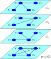
(Color online) An example of the difference between clustering coefficients. The local clustering coefficient of all nodes is 0 in each single layer, but 1 in the projection network.

Fig. 5

Schematic illustration of the monoplex network discussed in Section  2.3 and whose adjacency matrix is given in Table 1.

Fig. 6

(Color online) Schematic illustration of a two-layer multiplex network obtained by duplicating the network of Fig. 5, and connecting each node with its counterpart in the other layer.

Fig. 7

(Color online) Schematic illustration of a generic two-layer network with interlayer connections.

Fig. 8

(Color online) Schematic illustration of three kinds of correlated multiplex networks, maximally-positive (MP), uncorrelated (UC), and maximally-negative (MN). Each layer of the networks has different types of links, indicated by solid and dashed links, respectively.

Fig. 9

(Color online) Example of all possible multilinks in a multiplex network with $M=2$ layers and $N=5$ nodes. Nodes $i$ and $j$ are linked by one multilink $\overrightarrow{m}=(m_{\alpha },m_{{\alpha }^{\prime }})$.

Fig. 10

(Color online) Properties of multilinks in the weighted collaboration (layer 1)/citation (layer 2) multiplex network based on the PRE publications analyzed in Ref.  . In the case of the collaboration network, the distributions of multistrengths versus multidegrees always have the same exponent, but the average weight of multilinks $(1,1)$ is larger than the average weight of multilinks $(1,0)$. Moreover, the exponents ${\lambda }_{(1,0),col,in}$, ${\lambda }_{(1,0),col,out}$ are larger than exponents ${\lambda }_{(1,1),col,in},{\lambda }_{(1,1),col,out}$. In the case of the citation layer, both the incoming multistrengths and the outgoing multistrengths have a functional behavior that varies depending on the type of multilink. Conversely, the average inverse multiparticipation ratio in the citation layer does not show any significant change of behavior when compared across different multilinks.

Fig. 11

(Color online) Distributions $P\left(B_i\right)$ of the node-activity $B_i$ for (a) the six continental airline multiplex networks and for (b) APS and IMDb. Note that these distributions are broad and can be fitted by power-law exponents between 1.5 and 3.0 indicating that the typical number of layers in which a node is active is subject to unbound fluctuations.

Fig. 12

The network between 20 European airline companies in which each link is weighted with their layer pairwise multiplexity. This method can reveal non trivial correlations between the activities of the nodes in the different layers.

Fig. 13

(Color online) Panels (a)–(b): Degree distribution $P\left(k\right)$ in each layer (left), and the interlayer degree–degree correlations $\overline{k}\left(k\right)$ (right) for the case $c_{1,1}=1,c_{1,2}=0,c_{2,1}=0,c_{2,2}=1$ (top) and the case $c_{1,1}=0,c_{1,2}=1,c_{2,1}=1,c_{2,2}=0$ (bottom) attachment kernels (red circles are for the first layer, yellow squares for the second layer).

Fig. 14

(Color online) Phase diagrams of the non-linear multiplex network growing model. By means of a color code, the following quantities are plotted (see Ref.  for the definition of the plotted measures): (a) the number of distinct degree classes $\left|k\right|$, (b) the participation ratio $Y_2^{-1}$, and (c) the Kendall’s $\tau$ correlation coefficient. The solid black lines in panel (a) and (b) separate the non-condensed (region I) from the condensed phase (region II, small $\left|k\right|$, small $Y_2^{-1}$). In region I we can have either homogeneous (region I_a) or heterogeneous degree distributions (region I_b). The solid black line in panel (c) separates the two regions corresponding to positive (region $+,\tau >0$) or negative interlayer degree correlations (region $-,\tau <0$). The value of $\tau$ for the whole multiplex is negative only in region ${-}_b$. In panel (d) the plot of $\tau \left(t\right)$, which is the Kendall’s restricted to the nodes arrived up to time $t$ is shown. The dashed black line corresponds to $\tau =0$ and is reported for visual reference. For $\beta <0$ the interlayer correlations for older nodes are disassortative ($\tau \left(t\right)<0$ for small $t$), even if the value computed on all the nodes might be positive due to the prevalence of young nodes.

Fig. 15

(Color online) Schematic view of a typical network of networks with given supernetwork. Interdependencies (interlinks between nodes from different levels) are shown by the black dashed lines. Intralinks between nodes within layers are shown as solid red lines.

Fig. 16

(Color online) Schematic representation of a network of networks with given superdegree distribution. Each layer $\alpha$ has assigned given superdegree $q_{\alpha }$ but each node $(i,\alpha )$ can be linked to any $q_{\alpha }$ replica nodes.

Fig. 17

(Color online) Schematic representation of a network of networks with fixed supernetwork and random permutations of the labels of the nodes (case III). The supernetwork can be arbitrary but in the drawing we show a specific realization in which the supernetwork is a loop formed by $M=3$ layers.

Fig. 18

(Color online) Schematic representation of a network of networks with multiple interconnections. Each node $(i,\alpha )$ has $k_i^{\alpha \beta }$ links with nodes in layer $\beta$.

Fig. 19

Schematic description on how to find the mutually connected component in a multilayer interdependent network (duplex) considering the cascading failures propagating from one layer to the other one as described in Section  4.2. The set of active nodes that remains at the end of the cascade is the mutually connected component.

Fig. 20

(Color online) The function $g_{cp=y}(x=Sc)=x-y{(1-e^{-x})}^2$ plotted for different values of $y=cp$. The solution of the equation $g_{cp}\left(Sc\right)=0$ determines the fraction $S$ of nodes in the mutually connected component of a duplex formed by two Poisson networks with average degree $c$, when a fraction $1-p$ of nodes has been damaged. As $cp<2.45541\dots$, only the trivial solution $S=0$ exists, while at $cp=2.45541\dots$ a non trivial solution $S>0$ emerges discontinuously.

Fig. 21

The quantity $Sc$ as a function of the product $cp$, where $S$ is the fraction of nodes in the mutually connected component of a duplex network formed by two Poisson networks with average degree $c$, and $1-p$ is the fraction of nodes initially damaged in the multiplex network.

Fig. 22

Phase diagram (for $p=1$) of a multiplex formed by two Poisson networks (network A and network B) with average degrees ${〈k〉}_A=z_A$ and ${〈k〉}_B=z_B$ respectively.

Fig. 23

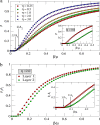
(Color online) Fraction of nodes $S$ in the MCGC as a function of $p$ for two symmetric power-law distributed networks with, from right to left, power-law exponent $\gamma =2.8,2.5$, and $\gamma =2.1$ and same minimal degree. The height of the jump becomes very small as the power-law exponent $\gamma$ approaches 2, but is not zero, as seen in the inset, which show $S$ vs. $p$ on a logarithmic vertical scale for $\gamma =2.1$.

Fig. 24

(Color online) Simulation results for the fraction of nodes $p_{\infty }=S$ in the mutually connected component as a function of $p$ for SF networks with power-law exponent $\lambda =3,2.7,2.3$, an ER network and a Random Regular (RR) network, all with an average degree $〈k〉=4$. The simulation results are performed at finite number of nodes $N$, and therefore are not clearly discontinuous due to finite size effects. Nevertheless, it can be seen already that $p_c$ is higher for broader distributions.

Fig. 25

(Color online) The fraction of nodes $p_n$ in the mutually connected component remaining after $n$ steps of the propagation of the damage back and forth between the two layers of a duplex network. In this case, the duplex has two layers with Poisson degree distribution and the same average $〈k〉$. Moreover, $p$ is set at the value $p=2.455/〈k〉<p_c$, and the total number of nodes $N$ is given by $N=12800$. The red circles indicate the theoretical predictions valid in the limit $N\to \infty$.

Fig. 26

(Color online) Simulation results for the fraction of nodes ${\beta }_{\infty }=S$ in the MCGC of a duplex formed by $N=50000$ nodes, as a function of $p$. For strong coupling (high value of $r$) between the networks, there is a discontinuity in ${\beta }_{\infty }$ (Poisson networks—circle, and SF networks—up rectangle). For weak coupling (low value of $r$) between the networks, the change in ${\beta }_{\infty }$ is described by a continuous transition (Poisson networks—square, and SF networks—right rectangle).

Fig. 27

Plots of the order parameter $\Sigma$ (left panel) and of the maximal superdegree of percolating layers $q_{max}$ (right panel) vs. $p$ for a configuration model with a Poisson $P\left(k\right)$ distribution with average $〈k〉=c=20$ and a SF $P\left(q\right)$ distribution with $\gamma =2.8$, and with minimal degree $m=1$ and maximal superdegree $Q={10}^3$.

Fig. 28

(Color online) Plot of ${\sigma }_q=S_q$ (fraction of nodes in a layer of superdegree $q$, belonging to the mutual component) vs. $p$ for different values $q=1,2,3$ in the configuration model of the network of networks having a Poisson $P\left(k\right)$ distribution with average $〈k〉=c=20$ and a SF $P\left(q\right)$ distribution with $\gamma =2.8$, minimal degree $m=1$ and maximal superdegree $Q={10}^3$. For each value of $q=1,2,3$, ${\sigma }_q$ emerges discontinuously, with a jump, which becomes smaller and smaller with increasing $q$. The emergence of ${\sigma }_2$ is accompanied by a discontinuity of ${\sigma }_1\left(p\right)$. The emergence of ${\sigma }_3$ is accompanied by discontinuities of ${\sigma }_1\left(p\right)$ and ${\sigma }_2\left(p\right)$.

Fig. 29

(Color online) The mutually connected component for a duplex of Poisson networks with different level of degree correlations. The symbol MP indicates maximally-positive degree correlations, the symbol MN indicates maximally-negative degree correlations, the symbol UC indicates no degree correlations.

Fig. 30

Phase diagram of the percolation of two antagonistic Poisson networks with average degree ${〈k〉}_A=z_A$ and ${〈k〉}_B=z_B$ for $p=1$. In region I none of the two networks is percolating. In Region II-A network A is percolating but not network B. Symmetrically, in region II-B network B is percolating but not network A. In region III there are two bistable solutions to the percolation problem and, depending on the initial conditions, either network A or network B is percolating.

Fig. 31

(Color online) Evolution of ${\lambda }_2\left(D_x\right)$ for multiplexes composed of two layers and $N={10}^3$. The layers are of the form: (a) scale-free (SF) with $P\left(k\right)\sim k^{-2.5}$ and Erdős–Rényi network with average degree $〈k〉=8$, (b) same SF network as in (a) and a Watts–Strogatz small-world network with $〈k〉=8$ and replacement probability of 0.3, (c) same SF network as in (a) and another SF network with $P\left(k\right)\sim k^{-3}$ and (d) same SF network as in (a) and the same SF network plus 400 additional links randomly placed. It is clear that in the first three examples superdiffusion shows up for large values of $D_x$, whereas for the multiplex in (d) this is not the case.

Fig. 32

(Color online) Evolution of ${\lambda }_2$ and its associated eigenvector, $v_2$, as a function of $D_x$ for a multiplex composed of two Erdős–Rényi networks of $N=50$ nodes and average degree $\overline{k}=5$. In this example, the critical point is ${\left(D_x\right)}_c=0.602\left(1\right)$. (a) Values of the components in $v_2$ (characteristic valuations) for the nodes in the two layers for $D_x=0.602$ (just before the onset of the transition). (b) ${\lambda }_2$ as a function of $D_x$ (black line). The discontinuity of the first derivative of ${\lambda }_2$ is very clear. The transition between the two known different regimes ($2D_x$, blue dashed line, and $\frac{{\lambda }_2(L^A+L^B)}{2}$, red dash-dotted line) is evident. (c) Projection of $v_2^B$ into $v_2^A$ as function of $D_x$. (d) Projection of the unit vector into $v_2^A$ and $v_2^B$ as functions of $D_x$. These two projections indicate the sum of all components of $v_2^A$ and $v_2^B$ respectively. (e) Values of the components in $v_2$ (characteristic valuations) for the nodes in the two layers for $D_x=0.603$ (just after the onset of the transition).

Fig. 33

(Color online) Path (sequence of arrows) of a random walker navigating a multiplex network composed of $N=7$ nodes and $M=3$ layers. In this example, the walker is neither allowed to switch between layer 1 and layer 3 in one time step nor to change node and layer simultaneously.

Fig. 34

(Color online) Evolution of the average Gene coefficient $〈G〉$ of the distribution of paths across the edges (left panel) and the average distance $〈\overline{d}〉$ between nodes (right panel) as functions of the average value of the interlayer coupling $〈\lambda 〉$ in the model introduced in Ref.  . The different curves correspond to different organization of the origin–destination matrix $T_{ij}$. This organization is initially centralized (one node is the unique destination of all the packets) and then randomized with some probability $p$. Reported data correspond to: $p=0$ (purple dots), 0.2 (blue squares), 0.4 (green diamonds), 0.6 (orange triangles), and 0.8 (red inverted triangles).

Fig. 35

(Color online) Panel (a): Fraction of infected individuals ($\rho$) at the steady state as a function of the control parameter $\frac{\beta }{\mu }$ for two interconnected networks of $N={10}^4$ nodes each for different values of the ratio $\eta =\frac{\delta }{\beta }$. The arrows show the inverse of the largest eigenvalues of the two coupled networks. The inset shows the case when the networks are uncoupled. In panel (b) the fraction of infected individuals is shown for each of the networks and for $\eta =2.0$. The inset is a zoom around the critical point showing how the epidemic in the second network is triggered by the onset in the first one.

Fig. 36

(Color online) The contour plot shows the epidemic threshold ${\beta }_c$ as a function of $\delta z$ and $\delta \lambda$ for a two layer multiplex composed of two ER networks. The dashed line (black) is a boundary of $\partial {\beta }_c/\partial \delta \lambda >0$ for all $\delta \lambda$, and the green (blue) line indicates the lowest (highest) value of ${\beta }_c$ at a given $\delta z$. ${\beta }_c$ shows non-monotonic dependence on $\delta \lambda$.

Fig. 37

(Color online) (Left panel) The survival regions diagram in the SI₁I₂S model in two-layer multiplex. Four possible scenarios appear: extinction region (N) where both viruses die-out, mutual extinction region I, where virus 1 survives and virus 2 dies out, mutual extinction region II, where only virus 2 survives and virus 1 dies out, and finally the coexistence region III, where both viruses survive and persist in the population. The red arrow shows the survival region of virus 1 (regions I and III) and the green arrow shows the survival region of virus 2 (regions II and III). (Middle and right panels) The two contour plots show the results from numerical simulations of the SI₁I₂S model for a multiplex composed of two SF networks of $N=1000$. The fraction of infected individuals in the steady state of the dynamics in network 1 (middle panel) and network 2 (right panel) are shown. The white lines are theoretical threshold curves accurately separating the survival regions as in the left panel.

Fig. 38

(Color online) Dependence of the onset of the epidemics ${\beta }_c$ as a function of $\lambda$ for different values of the recovery rates $\delta$ and $\mu$ for a two-layer multiplex composed of: (i) a SF network of $N=1000$ and exponent $2.5$ in the physical layer, where SIS dynamics takes place, and (ii) the same SF network of the physical layer plus 400 extra random links (non-overlapping with previous) in the virtual layer, where Aware–Unaware dynamics works. The shaded rectangle shows the free phase (in which all individuals are Unaware and Healthy) when the layers are uncoupled. The boundaries are defined by the bound of the structural characteristics of each layer: $1/\Lambda \left(A_1\right)$ and $1/\Lambda \left(A_2\right)$.

Fig. 39

Attack or adoption rate vs. the transmission probability in disease-only diffusion processes and coupled diffusion processes, where influenza is selected as the potential disease. Here, the adoption rate denotes the percentage of nodes adopting prevention behavior.

Fig. 40

(Color online) Snapshots of the evolution of opinion dynamics with three typical freezing periods $H$. From left to right, the values of $H$ are 0, 15 and 4000. In each panel, the vertical axis corresponds to the elapsed time, while the yellow and blue areas on the horizontal lines represent the opinion clusters. The total time spent to reach a global consensus, i.e. the consensus time $〈T〉$, under the scenario of intermediate value ($H=15$) is far less than two other cases. The size of networks is $N=500$, $q=0.01$ is the switching ratio during the freezing period. (For interpretation of the references to colour in this figure legend, the reader is referred to the web version of this article.)

Fig. 41

(Color online) Relationship between the normalized mean consensus time, $〈T〉/N$, and the number of interlayer links per node, $m/N$, for different network sizes. It is clear that there exist two consensus regimes. The solid line represents the relationship $〈T〉/N\propto {(m/N)}^{-1}$ as guides to the eye.

Fig. 42

(Color online) Fraction of cooperators $c$ in the population 1 as a function of $b$, for different values of the fraction $p$ of interpopulation contacts. The population 1 (of size $N_1={10}^3$) has been coupled to a smaller population 2 ($N_2={10}^2$). While initial strategies in population 1 are equally probable (random initial conditions), the population 2 starts from the absorbent state of fully defection. Other parameters are $r=0$, $ϵ=-0.4$. Both populations have a random (Erdős–Rényi) network of contacts with average degree $〈k〉=6$.

Fig. 43

(Color online) Cooperation diagrams of multinetworks. Average level of cooperation $〈c〉$ as a function of the temptation $b$ to defect for several multinetworks with different number of layers $M$ (the number of layers in indicated in the legend). In panel A the network layers are ER graphs with $〈k〉=3$ (sparse graphs) while in panel B we have $〈k〉=20$. In both cases $N=250$ nodes. As it can be observed, the resilience of cooperation increases remarkably as the number of layers $M$ grows.

Fig. 44

(Color online) Cross sections of phase diagrams for $\gamma =0.4$ (left) and $\gamma =0.9$ (middle) on the interdependent square lattices (green squares) and small-world networks (red triangles) with a fraction of rewired links equal to 0.05. The colored regions correspond to different sections: yellow is pure cooperators section, cyan is mixed strategies section, gray is pure defectors section and purple is symmetry breaking section. The lines in right panel denote the results of strategy-couple pair approximation for $\gamma =0.9$, which is qualitatively similar to the case of the middle panel. The dashed line represents an unstable solution of the analytical approach. Note that different ranges for the horizontal axis are used in the three panels, just for the guide of the eye.

Fig. 45

(Color online) The contour plots show the stationary fraction of cooperators $〈c〉$ as a function of the coupling parameters $\gamma$ and ${\gamma }^{\prime }$ entering in Eq. (230) for $r=3.5$ in PGG (left panel). Time courses of strategy pairs within and between networks (right panel), where $P_i$ and $P_e$ denote the corresponding pair configuration probabilities within (internal) and between (external) networks, respectively. The parameters are $r=3.5$, $\gamma =0.15$ and ${\gamma }^{\prime }=0.5$ in right panel.

Fig. 46

(Color online) The contour plots show the stationary fraction of cooperators $〈c〉$ as a function of the coupling ratio $\rho$ and coupling degree $\gamma$ for different cases. Both top panels and the left bottom one refer to a prisoner dilemma underlying game, whereas the snowdrift game is used in the bottom right panel. Square lattices are used except for the bottom left panel, which uses triangle lattices. Similarly, the top right panel uses proportion imitation rule  , , while Fermi update rule  , is held in the other ones. It is obvious that the proposed scenario of partial overlap is universally effective.

Fig. 47

(Color online) Strength distributions $P\left(s\right)$ of the commuting layers. (a) Initial condition $G_0$ (solid black line), $G\left(t\right)$ constructed by the eigenvalue surrogate method (thick solid red line), and $\Lambda \left(t\right)$ obtained by randomly choosing the eigenvalues from $p\left({\lambda }_0\right)$ in an ordered way (dashed blue line). (b) Eigenvalues randomly chosen from $p\left({\lambda }_0\right)$ in a unordered way (solid black line), eigenvalues chosen from a uniform distribution in an ordered way (thick solid red line), and in a unordered way (dashed blue line). The details of the statistical ensembles are the same as for Table 5.

Fig. 48

Time evolution of synchronization error $〈\delta 〉$ for $\tau =0.2$ (empty circles), 0.3 (filled circles), 0.4 (empty squares), 0.5 (filled squares), 0.6 (empty diamonds), 0.7 (filled diamonds), 0.9 (empty up triangles), 1.1 (filled up triangles), and 1.5 (empty down triangles). In all cases, the results are ensemble averages over 5 different random initial conditions for a dynamical network of $N=200$ identical chaotic Rössler oscillators. Inset: Synchronization time $T_{sync}$vs. switching time $\tau$ (open circles refer to different initial conditions, solid line is the ensemble average).

Fig. 49

Example of label swapping. Going from the basis on the left to the one in the middle while keeping $x$ constant necessarily involves a reflection. However, going from the basis on the right to the one in the middle can be accomplished via a proper rotation.

Fig. 50

(Color online) Targetability of different topologies. Targeting scheme for ER and SF networks of $N=500$ Rössler oscillators. The top panel shows ${\lambda }_{\max }$ as a function of the targeting step, for degree ranking and random ranking. The zero level is highlighted as a black horizontal line. The bottom panel shows the synchronization error vs. the targeting step. The legend contains the symbol codes for the specific topologies considered, as well as for the specific ranking used for the targeting. All results correspond to ensemble averages over 40 different graph realizations, and, for the random ranking case over 40 different ranking realizations.

Fig. 51

Link overlap (Jaccard coefficient), degree correlation and rank correlation for all pairs of layers in the Pardus social game network. E, enmity; F, friendship; A, attack; T, trade; C, communication; and B, bounty. Pairs of equal connotation (positive–positive and negative–negative) are marked with a gray background.

Fig. 52

Example of a space-based network. The two light gray boxes represent two spacecrafts, connected through a high-capacity communication system. Each one of them is composed of different modules, e.g. the Telemetry, Tracking and Command (TTC): when one of them fails, the corresponding spacecraft can rely on the other to backup that function, and to fulfill its mission.

Fig. 53

(Color online) Outcome of the re-scheduling process in the multilayer air transport network, as a function of the probability of link failure, $p$, and load tolerance, $f_{tol}$. Each column displays (from top to bottom): the average fraction of passengers that cannot fly, that of those that are re-scheduled in other layers, and that for those re-scheduled within the original layer. Each column accounts for the possibility of scheduling passengers on paths with length 0 (left), 1 (center), and 2 (right).

Fig. 54

(Color online) Example of an heterogeneous mobile communication network. The battlefield can be seen as a set of resources, e.g. tanks, soldiers, or even satellites, which require to continuously transmit tactical information to the others. Due to the different characteristics and capabilities of each resource, multiple communication networks are deployed (as, for instance, satellite, UHF or VHF links), making the system a multilayer network.

Fig. 55

(Color online) Commodity diversity and nodal regions in the maritime flow network. Nodes represent ports, pairwise connected by links when a commodity is transported between them. Different commodities are considered, thus making this graph a multilayer network. In order to represent this heterogeneity, links are colored according to the number of commodity types traveling between ports. Furthermore, both nodes and links sizes represent the corresponding traffic share.

Fig. 56

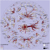
(Color online) Communities in the dream interpretation network: English (left), Chinese (center), and Arabic (right). Symbols with the highest eigenvector centrality are used to label each community. The complete networks are illustrated in the upper right corners of each figure, with colors corresponding to the communities (colors are not intended to match across different networks).

References

1. Strogatz S.H. Exploring complex networks. Nature. 2001;410(6825):268–276. doi: 10.1038/35065725. - DOI - PubMed
1. Albert R., Barabási A.-L. Statistical mechanics of complex networks. Rev. Mod. Phys. 2002;74(1):47–97. doi: 10.1103/RevModPhys.74.47. - DOI
1. Dorogovtsev S.N., Mendes J.F. Evolution of networks. Adv. Phys. 2002;51(4):1079–1187. doi: 10.1080/00018730110112519. - DOI
1. Newman M. The structure and function of complex networks. SIAM Rev. 2003;45(2):167–256. doi: 10.1137/S003614450342480. - DOI
1. Watts D. Princeton University Press; Princeton, NJ, USA: 1999. Small Worlds: The Dynamics of Networks Between Order and Randomness.