COVID-19 and SARS-CoV-2. Modeling the present, looking at the future

Abstract

Since December 2019 the Severe Acute Respiratory Syndrome Coronavirus 2 (SARS-CoV-2) has produced an outbreak of pulmonary disease which has soon become a global pandemic, known as COronaVIrus Disease-19 (COVID-19). The new coronavirus shares about 82% of its genome with the one which produced the 2003 outbreak (SARS CoV-1). Both coronaviruses also share the same cellular receptor, which is the angiotensin-converting enzyme 2 (ACE2) one. In spite of these similarities, the new coronavirus has expanded more widely, more faster and more lethally than the previous one. Many researchers across the disciplines have used diverse modeling tools to analyze the impact of this pandemic at global and local scales. This includes a wide range of approaches - deterministic, data-driven, stochastic, agent-based, and their combinations - to forecast the progression of the epidemic as well as the effects of non-pharmaceutical interventions to stop or mitigate its impact on the world population. The physical complexities of modern society need to be captured by these models. This includes the many ways of social contacts - (multiplex) social contact networks, (multilayers) transport systems, metapopulations, etc. - that may act as a framework for the virus propagation. But modeling not only plays a fundamental role in analyzing and forecasting epidemiological variables, but it also plays an important role in helping to find cures for the disease and in preventing contagion by means of new vaccines. The necessity for answering swiftly and effectively the questions: could existing drugs work against SARS CoV-2? and can new vaccines be developed in time? demands the use of physical modeling of proteins, protein-inhibitors interactions, virtual screening of drugs against virus targets, predicting immunogenicity of small peptides, modeling vaccinomics and vaccine design, to mention just a few. Here, we review these three main areas of modeling research against SARS CoV-2 and COVID-19: (1) epidemiology; (2) drug repurposing; and (3) vaccine design. Therefore, we compile the most relevant existing literature about modeling strategies against the virus to help modelers to navigate this fast-growing literature. We also keep an eye on future outbreaks, where the modelers can find the most relevant strategies used in an emergency situation as the current one to help in fighting future pandemics.

Fig. 1.1

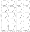
Evolution of the number of confirmed cases in the world since December 31th 2019 until June 19th 2020. Notice the logarithmic scale on the y-axis displaying the number of confirmed cases.

Fig. 1.2

Evolution of the COVID-19 pandemic across the world since January 2020 until Jun 2020.

Fig. 1.3

Schematic representation of the main transmission route of SARS CoV-2 between individuals (see further for indirect transmission). The graphic was prepared using Motifolio.

Fig. 2.1

Illustration of a weighted graph (left) and a multilayer graph (right).

Fig. 2.2

Prediction made by Prasse et al.  for the outbreak in Hubei for 4 cities. Reproduced with permission by the authors.

Fig. 2.3

Illustration of the mobility network of the European Union (left), and of the effects of travel restrictions according to Linka et al. . Figures provided by the authors.

Fig. 2.4

Illustration of a multiplex formed by two layers $i$ and $j$. Notice that the set of vertices is the same in each of the two graphs $G_i$ and $G_j$, but not the sets of edges $E_i\ne E_j$.

Fig. 2.5

Illustration of the results obtained by Chung and Chew  for the dynamical evolution of the reproduction number with and without circuit breaker (CB) (a), and with and without gradual lifting (G) (b) measures. Figures provided by the authors.

Fig. 2.6

Illustration of a metapopulation network.

Fig. 2.7

Comparison of the spreading from the two major cities of Spain at to different times as reported by Aleta and Moreno . The reported values are the median over 103 simulations. The figure is reproduced with permission from the authors.

Fig. 2.8

Schematic illustration of the indirect transmission of COVID-19. An individual sneeze or cough over a surface (left), which is then touched by another individual (center) who brings the virus from her hands to her respiratory system (right).

Fig. 2.9

Scheme of the compartments used in the model developed by Godio et al. .

Fig. 2.10

Results of the simulations reported by Eikenberry et al.  for the cumulative death tolls for Washington state (top panels) and New York (bottom panels), using a fixed transmission rate, and different permutations of general public mask coverage and effectiveness. Reproduced with permission.

Fig. 2.11

Scheme of the compartments used in the model developed in , , .

Fig. 2.12

Contribution of cases from the 10 Chinese cities with the highest rates of disease to the relative risk of importation in different countries before (left) and after (right) travel ban in Wuhan as reported by Chinazzi et al. .

Fig. 2.13

Modeling scheme of work of Aleta et al.  where the weighted multilayer synthetic population is built from mobility data in the metropolitan area of Boston (a). The agent-based system of adults and children, whose geographical distributions (b). The compartmental model used (c) where the description of the variables is given in the text. Figure provided by the authors.

Fig. 2.14

Scheme of the compartment model used by Arenas et al. , . Figure provided by the authors.

Fig. 2.15

Illustration of the results reported by Arenas et al.  for each autonomous region in Spain. The solid line is the result of the epidemic model, aggregated by ages, for the number of individuals inside compartments (H+R+D) that corresponds to the expected number of cases, and dots correspond to real cases reported. Figure provided by the authors.

Fig. 2.16

Left: Value of the effective reproduction number, $\mathcal{R}\left(t_c\right)$, when containment measures are taken as a function of the confinement ${\kappa }_0$ and social distancing $\delta$ computed from Eq. (2.17). Right: Evolution of new cases for different values of confinement ${\kappa }_0$ when social distancing is fixed to $\delta =0.4$.

Fig. 2.17

Illustration of the weighted in- and outdegree distributions of the directed graph studied by . Figure provided by the authors.

Fig. 2.18

Forecasts made by Perc et al.  of COVID-19 cases for the United States, Slovenia, Iran, and Germany. Black solid line denotes the actual data, which were for this analysis last updated on​ March 29th. The different output scenarios are displayed in different colors: nothing would change (solid blue line); maximal daily growth rate increased by 20% (solid red line); daily growth rate would drop to zero (green line); equally spaced decreasing daily growth rates from top to bottom (orange and olive dashed lines). Figure reproduced with permission of the authors.

Fig. 2.19

Fit to data for the daily number of active cases in Spain from March 1st to March 29th as reported by Castro et al. . The solid line represents estimation using the median parameters for each posterior in the model. The shaded area represents the 95% predictive posterior interval. Inset: same data and curves with linear vertical scale. The figure is reproduced with permission of the authors.

Fig. 3.1

Illustration of the life cycle of the SARS CoV-2 based on current knowledge. The graphics were prepared using Motifolio (https://www.motifolio.com/).

Fig. 3.2

Crystal structures of 3CL protease (a), papain-like protease (b), nsp15 endoribonuclease (c), nsp12–nsp7–nsp8 complex bound to the template-primer RNA (d) and nsp16-nsp10 heterodimer (e) with inhibitors. The inhibitors are marked with a yellow arrow. The PDB structures correspond, respectively, to: 6Y2G , 6WX4 , 6WXC , 7BV2  and 6WKQ (to be published).

Fig. 3.3

Illustration of protein–ligand binding induced topological fingerprints change as reported by Cang and Wei . Figure provided by the authors.

Fig. 3.4

Cartoon representation (left) of the M^pro of SARS CoV-2 (PDB ID: 6Y2E) and the corresponding protein residue network (right).

Fig. 3.5

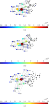
Illustration of the 22 amino acids with the largest values of the long-range subgraph centrality in 6M0K (a), 6LZE (b) and 6Y2G (c). The residues are connected if they are at no more than 7.0 Å. The color bar and the radius of the nodes indicates the values of $Z_{ii}$ normalized to the largest value in the corresponding protein.

Fig. 3.6

3D structure of the complex between nsp10 and S-adenosyl-L-methionine (SAM) (PDB ID: 6W4H).

Fig. 3.7

Complexes of vapreotide (a) and atazanavir (b) with SARS CoV-2 helicase protein built from molecular homology reproduced from Borgio et al. .

Fig. 3.8

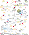
Illustration of the PPIs of SARS-CoV-2 baits with approved drugs (green), clinical candidates (yellow), and preclinical candidates (purple) with experimental activities against the host proteins (white background) or previously known host factors (gray background). Figure provided by the authors.

Fig. 4.1

Global scheme of vaccine development pipeline.

Fig. 4.2

Proposed scheme for anti-SARS CoV-2 vaccine development.

Fig. 4.3

The main steps of the rational vaccine design pipeline adapted from a diagram in  and made using Motifolio.

Fig. 4.4

Composition of the structures of SARS CoV-2 S protein, ACE2 receptor and neutral amino acid transporter B0AT1 forming the entry complex of the virus into the human cell.

Fig. 4.5

Molecular and cellular mechanism of immune responses induced against SARS CoV-2. Graphics prepared with Motifolio.

Fig. 4.6

Illustration of the key interactions obtained from the structure of TLR3 and vaccine complex, before (A) and after (B) molecular dynamics simulation. TLR3 receptor is shown in green color, and the vaccine is shown in cyan color in both panels .

References

1. Cheng V.C., Lau S.K., Woo P.C., Yuen K.Y. Severe acute respiratory syndrome coronavirus as an agent of emerging and reemerging infection. Clin. Microbiol. Rev. 2007;20(4):660–694. - PMC - PubMed
1. Richard M., Kok A., de Meulder D., Bestebroer T.M., Lamers M.M., Okba N.M., van Vlissingen M.F., Rockx B., Haagmans B.L., Koopmans M.P., et al. SARS-CoV-2 is transmitted via contact and via the air between ferrets. Nat. Commun. 2020;11:3496. - PMC - PubMed
1. Bar-On Y.M., Flamholz A., Phillips R., Milo R. Science forum: SARS-CoV-2 (COVID-19) by the numbers. Elife. 2020;9 - PMC - PubMed
1. Rothan H.A., Byrareddy S.N. The epidemiology and pathogenesis of coronavirus disease (COVID-19) outbreak. J. Autoimmun. 2020;109 - PMC - PubMed
1. Vannabouathong C., Devji T., Ekhtiari S., Chang Y., Phillips S.A., Zhu M., Chagla Z., Main C., Bhandari M. Novel coronavirus COVID-19: current evidence and evolving strategies. J. Bone Joint Surg. 2020;102(9):734. - PMC - PubMed