Complete dimensional collapse in the continuum limit of a delayed SEIQR network model with separable distributed infectivity

Abstract

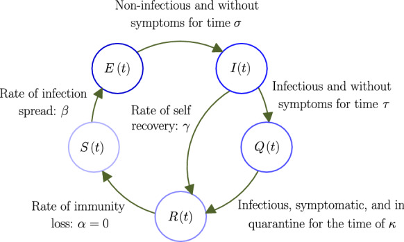
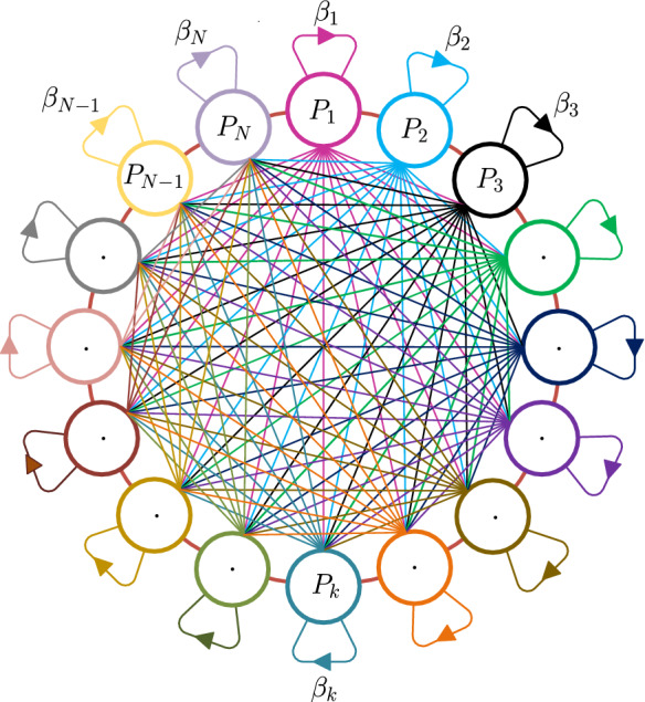
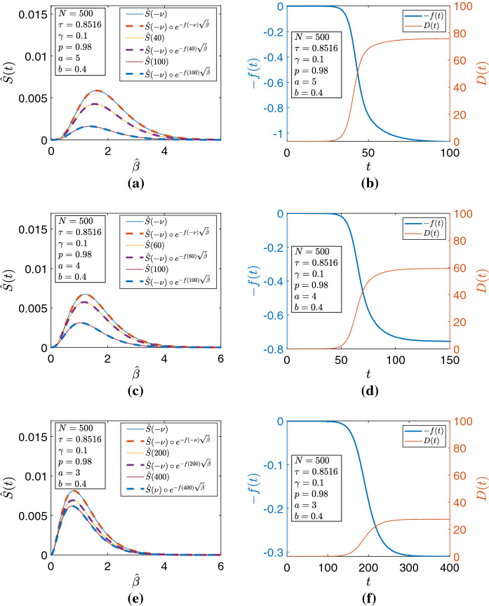
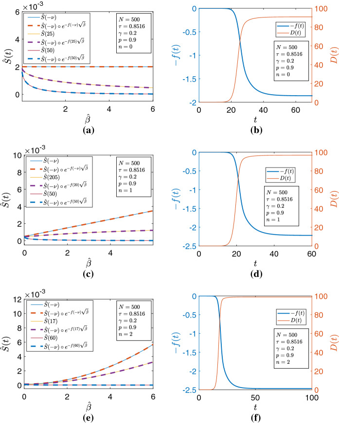
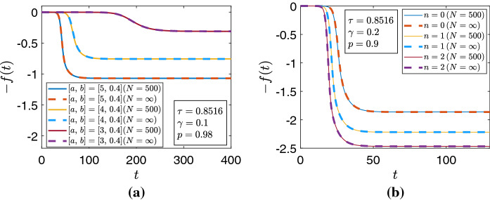
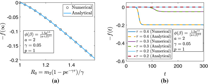
We take up a recently proposed compartmental SEIQR model with delays, ignore loss of immunity in the context of a fast pandemic, extend the model to a network structured on infectivity and consider the continuum limit of the same with a simple separable interaction model for the infectivities $\beta$ . Numerical simulations show that the evolving dynamics of the network is effectively captured by a single scalar function of time, regardless of the distribution of $\beta$ in the population. The continuum limit of the network model allows a simple derivation of the simpler model, which is a single scalar delay differential equation (DDE), wherein the variation in $\beta$ appears through an integral closely related to the moment generating function of $u=\sqrt{\beta }$ . If the first few moments of u exist, the governing DDE can be expanded in a series that shows a direct correspondence with the original compartmental DDE with a single $\beta$ . Even otherwise, the new scalar DDE can be solved using either numerical integration over u at each time step, or with the analytical integral if available in some useful form. Our work provides a new academic example of complete dimensional collapse, ties up an underlying continuum model for a pandemic with a simpler-seeming compartmental model and will hopefully lead to new analysis of continuum models for epidemics.

Keywords: COVID-19; Epidemic; Pandemic; Reduced order; Time delay.

Fig. 1

The SEIQR compartmental model with delays

Fig. 2

A schematic representation of N interacting population groups with different infection spread rates among each group. Every connection between two groups is bidirectional and symmetric, and every group is connected to all other groups (a dense network)

Fig. 3

Simulations with different initial values $\widehat{S}(-\nu )$. Here, a Gamma distribution is used for $\widehat{U}(\widehat{\beta })=\frac{1}{b^a\Gamma (a)}{\widehat{\beta }}^{(a-1)}{e}^{\frac{-\widehat{\beta }}{b}}$, along with $\widehat{V}(\widehat{\beta })=\widehat{U}(\widehat{\beta })$. Also shown is the fit of the form of Eq. (19) at different instants of time. We note that as the $\beta$ values in the distribution get smaller on average, $D(\infty )$ decreases

Fig. 4

Simulations with different initial values $\widehat{S}(-\nu )=\widehat{U}(\widehat{\beta })$. Here, finitely supported polynomials of the form $\widehat{U}(\widehat{\beta })=r_n·\left(1,+,{\widehat{\beta }}^n\right),0\le \widehat{\beta }\le 6$ are considered, with $r_n$ chosen to make the sum (or 1-norm) of $\widehat{U}(\widehat{\beta })$ equal to 1. The distribution of initial values for $\widehat{I}(\widehat{\beta })$ uses $\widehat{V}(\widehat{\beta })$ that is random, initially uniformly distributed between 1 and 2, and then normalized to unit 1-norm. Also shown is the fit $\widehat{S}(t)=\widehat{S}(-\nu )\circ e^{-f(t)\sqrt{\widehat{\beta }}}$ at different instants of time. These results demonstrate that provided the initial infected population distribution is small, the subsequent evolution obeys a simple one-dimensional description with a scalar variable f(t)

Fig. 5

Comparison between the continuum solution $-f(t)$ of Eq. (33) and the discrete network solution [Eqs. (15) and (16)] with $N=500$ fitted using $\widehat{S}(t)=\widehat{S}(-\nu )\circ e^{-f(t)\sqrt{\widehat{\beta }}}$. a $\widehat{U}(\widehat{\beta })=\frac{1}{b^a\Gamma (a)}{\widehat{\beta }}^{(a-1)}{e}^{\frac{-\widehat{\beta }}{b}}$ and $\widehat{V}(\widehat{\beta })=\widehat{U}(\widehat{\beta })$. b $\widehat{U}(\widehat{\beta })=r_n·(1+{\widehat{\beta }}^n),0\le \widehat{\beta }\le 6$ and $\widehat{V}(\widehat{\beta })$ randomized as in Fig. 4. The history function for Eq. (33) is taken as $f(t)=\omega \times (1+\frac{t}{\nu })$, with $\omega$ is adjusted to match the results from [Eqs. (15) and (16)]. Other numerical parameters are mentioned in text boxes within subplots

Fig. 6

An example with unbounded moment $m_3$ (see Eq. (50)). a $R_0$ on the horizontal axis governs stability. Each circle, labeled “numerical,” represents the saturation value observed in a numerical solution based on integration of Eq. (33) combined with Eq. (39). At every time step, the integral in Eq. (39) is evaluated numerically for the truncated domain $0<u<1000$. The continuous line labeled “analytical” is from Eq. (33) with Eq. (51) used directly. b Comparison of time responses $-f(t)$, with “numerical” and “analytical” implying the same as in (a). The initial function used was $f(t)=1\times {10}^{-9}+1\times {10}^{-9}\left(1,+,\frac{t}{\nu }\right),t\le 0$

References

-
- Kermack WO, McKendrick AG. A contribution to the mathematical theory of epidemics. Proc. R. Soc. Lond. A Math. Phys. Eng. Sci. 1927;115(772):700–721.
- Hethcote, H.W.: The basic epidemiology models: models, expressions for R0, parameter estimation, and applications. In: Ma, S., Xia, Y. (eds.) Ma, S., Xia, Y. (eds.) Mathematical Understanding of Infectious Disease Dynamics, pp. 1–61. World Scientific (2009)
- Brauer F, Castillo-Chavez C, Castillo-Chavez C. Mathematical models in population biology and epidemiology. New York: Springer; 2012.
- Hethcote HW. The mathematics of infectious diseases. SIAM Rev. 2000;42(4):599–653. doi: 10.1137/S0036144500371907. - DOI
LinkOut - more resources
Full Text Sources