Low-dimensional dynamics for working memory and time encoding

Abstract

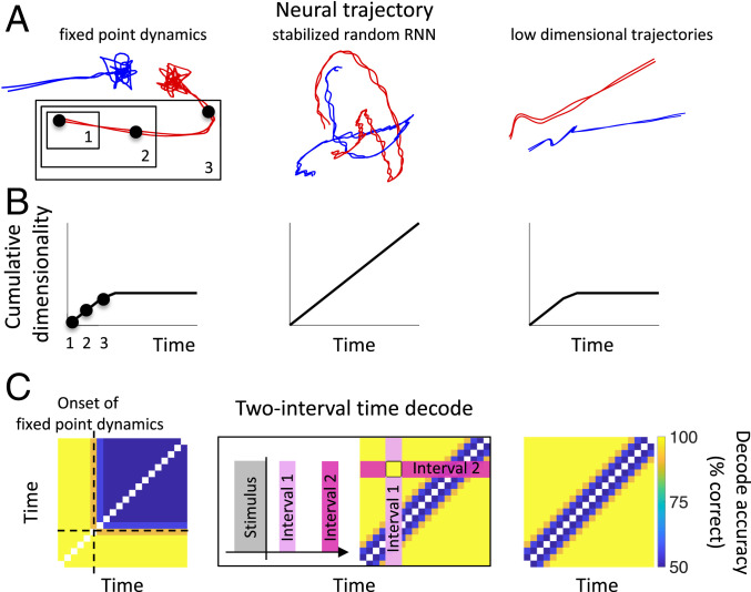
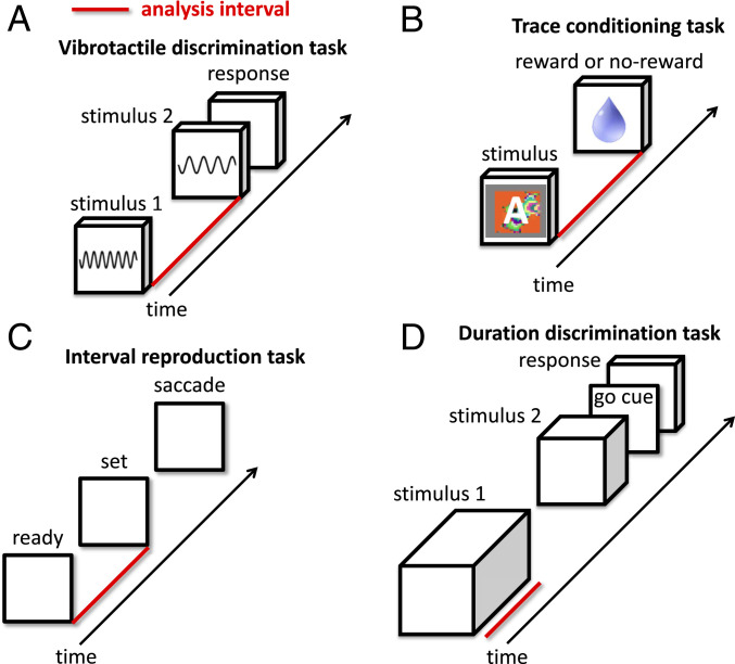
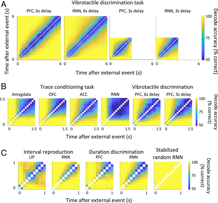
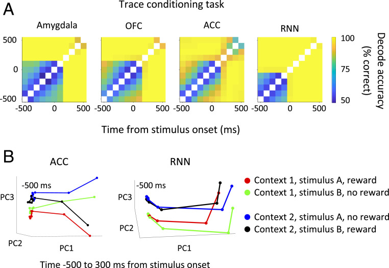
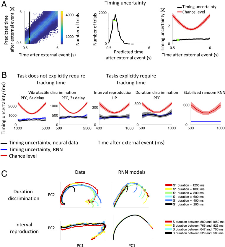
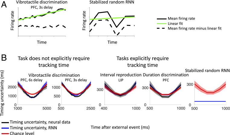
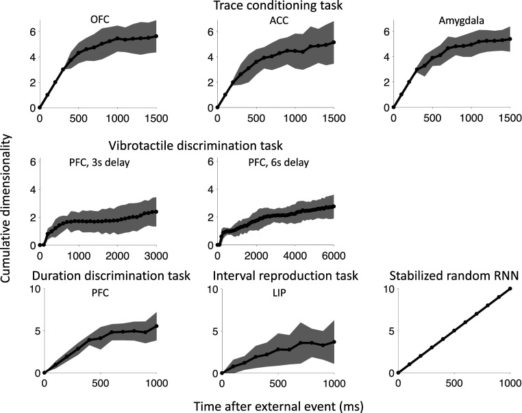
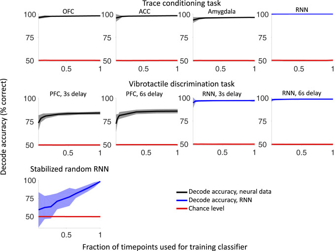
Our decisions often depend on multiple sensory experiences separated by time delays. The brain can remember these experiences and, simultaneously, estimate the timing between events. To understand the mechanisms underlying working memory and time encoding, we analyze neural activity recorded during delays in four experiments on nonhuman primates. To disambiguate potential mechanisms, we propose two analyses, namely, decoding the passage of time from neural data and computing the cumulative dimensionality of the neural trajectory over time. Time can be decoded with high precision in tasks where timing information is relevant and with lower precision when irrelevant for performing the task. Neural trajectories are always observed to be low-dimensional. In addition, our results further constrain the mechanisms underlying time encoding as we find that the linear "ramping" component of each neuron's firing rate strongly contributes to the slow timescale variations that make decoding time possible. These constraints rule out working memory models that rely on constant, sustained activity and neural networks with high-dimensional trajectories, like reservoir networks. Instead, recurrent networks trained with backpropagation capture the time-encoding properties and the dimensionality observed in the data.

Keywords: neural dynamics; recurrent networks; reservoir computing; time decoding; working memory.

Fig. 1.

Three hypotheses for neural dynamics, which can be disambiguated by decoding time and dimensionality. (A) Trajectories in the firing-rate space: the firing rates of a population of simulated neurons are shown after they have been projected onto a two-dimensional space. (Left) A transient response is followed by fixed-point dynamics. Information about two behavioral states is stored in separate fixed points colored in red and blue. The two lines for each behavioral state correspond to two different trials. These fixed points are attractors of the dynamics, and the fluctuations around them are due to noise. (Center) A randomly connected “reservoir” of neurons generates chaotic trajectories. The trajectories have been stabilized as in Laje and Buonomano (17). The neural activity at each time point is unique, and these changing firing rates can be used as a clock to perform different computations at different times. Importantly, the red and blue trajectories are distinct and linearly separable for all times, so the behavioral state is also encoded throughout the interval. (Right) Low-dimensional trajectories: a transient is followed by linearly ramping neural responses. (B) To compute the cumulative dimensionality, the neural trajectory is first subdivided into nonoverlapping intervals (three example intervals are highlighted with black dots in A). The cumulative dimensionality at time $t$ is the dimensionality of the neural trajectory spanning intervals 1 through $t$ (see SI Appendix, Fig. S1 for details). The cumulative dimensionality of the neural activity over time increases linearly in the standard stabilized random RNN (Center). This is in contrast to fixed-point and ramping dynamics, where the cumulative dimensionality increases during an initial transient and then plateaus during the fixed-point and ramping intervals. These two dynamical regimes yield the same cumulative dimensionality; however, they are disambiguated by computing the two-interval time decode. (C) Two-interval time-decode matrix for the simulated data shown in A. Subdivide the time after stimulus offset into nonoverlapping intervals. Take the vector of firing rates recorded from all neurons during a single interval (interval 1 after stimulus offset, for example), and train a binary classifier to discriminate between this and another interval (interval 2). Test the classifier on held-out trials and record the performance. This number, between 50 and 100%, from the classifier trained to discriminate intervals i and j is recorded in pixel (i,j) of the “two-interval time-decode matrix.” If the decode accuracy is 100%, the pixel is colored yellow (as shown in the example in Center), and if the decode accuracy is 50%, the pixel is colored blue. (Left) The block of time where the decode is near chance level (50%) is a signature of fixed-point dynamics; once the fixed point is reached, a classifier cannot discriminate different time points. In contrast, for the stabilized random RNN and low-dimensional trajectories, it is possible to decode time (down to some limiting precision due to noise in the firing rates).

Fig. 2.

Four tasks analyzed in this paper. Red bars indicate time intervals that were analyzed. To better understand neural dynamics in the absence of external events, we only analyzed intervals with over 1,000 ms between changes in sensory stimuli. (A) In the vibrotactile-discrimination task of Romo et al. (38), a mechanical probe vibrates the monkey’s finger at one of seven frequencies. Then, there is either a 3- or 6-s delay interval before the monkey’s finger is vibrated again at a different frequency. The monkey’s task is to report whether the frequency of the second stimulus is higher or lower than that of the first. (B) In the context-dependent trace-conditioning task of Saez et al. (39), monkeys were presented with one of two visual stimuli, A or B. After a 1.5-s delay period, the monkey was either rewarded or not. This is a context-dependent task: in context 1, stimulus A is rewarded and stimulus B is not, whereas, in context 2, the associations are reversed (stimulus A is not rewarded and stimulus B is rewarded). Monkeys learned the current context and displayed anticipatory licking after the appropriate stimuli. (C) In the ready-set-go interval-reproduction task of Jazayeri and Shadlen (41), the monkey tracks the duration between ready and set cues in order to reproduce the same interval with a self-initiated saccade at the appropriate time after the set cue. The interval between ready and set cues was at least 1 s for all analyses. (D) In the duration-discrimination task of Genovesio et al. (42), the monkey compares the duration of two stimuli and then reports which stimulus was on longer. The duration of stimulus 1 was at least 1 s for all analyses.

Fig. 3.

Two-interval time decode. (A) The two-interval time-decode analysis for the vibrotactile-discrimination task for delay intervals of 3 and 6 s is shown for both the data and RNN model. The longer delay-period intervals used in this task reveal neural dynamics that evolve slowly, on a timescale of approximately half a second (see also Fig. 5B). Time can be decoded but with limited precision. (B) Two-interval time-decode matrices for the vibrotactile-discrimination task and trace-conditioning task are similar during the delay interval after stimulus offset, when truncating the vibrotactile dataset to match the 1,500-ms delay interval used in the trace-conditioning task. The similarities in these two datasets suggest the observations in the trace-conditioning task are compatible with a slowly varying dynamics, which have been truncated due to the shorter 1,500-ms delay interval used in this experiment (see also SI Appendix, Fig. S12). (C) Two-interval time-decode matrices for the interval-reproduction task (41), duration-discrimination task (42), and stabilized random RNN (17) reveal that time is encoded with higher precision in tasks that explicitly require tracking time. Times are aligned to the ready cue for the interval-reproduction task, S1 onset for the duration-discrimination task, and stimulus offset for the stabilized random RNN. There are no external events during the 1,000-ms interval over which the two-interval time decode is shown, i.e., no external inputs or visual stimuli were changed during this 1,000-ms interval.

Fig. 4.

Decoding time from neural activity reveals signatures of fixed-point dynamics. (A) Pixel (i,j) is the decode accuracy of a binary classifier trained to discriminate time points i and j using 100-ms bins of neural activity. The blocks of time where the decode is near chance level (50%) are signatures of fixed-point dynamics. The pattern of fixed points seen in the data agrees with the RNN model. In the model, the fixed points before stimulus onset store contextual information. Importantly, a linear classifier can easily discriminate other task-relevant quantities during these time intervals so the poor time decode is not simply due to noisy neural responses that have lost all informational content (SI Appendix, Fig. S10). (B) The average neural trajectories for all four trial types are plotted on the three principal components capturing most of the variance. Time is discretized in 100-ms nonoverlapping bins (denoted by dots) and shown from −500 to 300 ms relative to stimulus onset. During the fixed-point interval before stimulus onset, the trajectories cluster according to context.

Fig. 5.

(A) To quantify the precision with which time is encoded, we estimated the temporal uncertainty at each point in time by training a classifier to report the time point a neural recording was made and then compare this prediction with the actual time (SI Appendix, Fig. S3); we repeat this classification for many trials, obtaining a distribution about the true time. Left shows the distribution of predicted versus actual times for the vibrotactile-discrimination task, excluding the initial transient after stimulus offset. The distribution of predictions at a single time point, marked by the vertical black line, is replotted in Center. The green bar shows the SD of this distribution. The “timing uncertainty” is the SD of this distribution and contributes a single data point to the “timing uncertainty” graph (Right) (green dot). The timing uncertainty for all time points is shown in black. The chance level is shown in red. (B) The timing uncertainty for the neural data (black curves) and RNN models (blue curves) is less than chance level (red curves) and has better resolution for tasks in which timing information is explicitly required, as in the duration-discrimination task and the ready-set-go interval-reproduction task (note the scales on the y axes are different). This is consistent with the idea that stable neural trajectories act as a clock to perform the task. Error bars show two SDs. (C) Visualization of these putative neural clocks after projecting the neural activity onto the first two principal components capturing the most variance. The left column shows the data for the two tasks that require keeping track of time, and the right column shows the RNN models. Trajectories show the intervals when time is being tracked. For the duration-discrimination task, this is the interval when stimulus one (S1) is on the screen. For the interval-reproduction task, this is the “sample” interval between ready and set cues, denoted by S in the figure legend. Colors indicate the duration of the interval. To better visualize these neural clocks, we include data from all durations, not just durations over 1,000 ms as in B. Principal axes were computed using only data from the longest duration (red curves; first principal component explains over 50% of the variance for all datasets and models), and then data from the shorter durations were projected onto these axes. The black crosses plotted on the trajectories of the duration-discrimination task indicate when the visual stimulus changed to indicate when the monkey should stop counting the duration of the interval, i.e., S1 offset. After this cue, the neural activity gets off the “clock.” All neurons were included that were recorded for 10 or more trials for each duration.

Fig. 6.

The linear ramping component of each neuron’s firing rate drives the decoder’s ability to estimate the passage of time (compare with Fig. 5). (A) For each neuron, we calculate the linear fit to the average firing rate across trials during the same time interval as in Fig. 5. We then subtract this linear fit from the firing rate on every single trial and calculate the timing uncertainty. (B) After the linear ramping component is removed, the timing uncertainty in both the neural data (black curves) and trained RNN models (blue curves) is near chance level (red curves). In contrast, for the untrained RNN with stabilized chaotic dynamics (17), it is still possible to decode time with high accuracy, down to the limiting resolution set by the 100-ms time bin of the analysis, even after the linear component has been removed. Error bars show two SDs.

Fig. 7.

The cumulative dimensionality of the neural activity increases slowly over time after a transient of ∼500 ms. In contrast, the cumulative dimensionality increases linearly in the stabilized random network (17). The top and middle rows show dimensionality for tasks in which timing is not explicitly important. The bottom row shows dimensionality for tasks in which timing is required. The cumulative dimensionality for the RNN models is similar and is shown in SI Appendix, Fig. S14. Error bars show two SDs.

Fig. 8.

Decode generalization when classifying neural activity with low and high cumulative dimensionality. The decode accuracy of a binary classifier (colored in black for data and blue for RNN models) is shown as the number of time points used during training is varied. The chance level is shown in red. The neural activity with low cumulative dimensionality allows a classifier trained at a single time point to perform with high accuracy when tested at other times. This is in contrast to neural activity with high cumulative dimensionality (bottom row) where a decoder trained at a single time point performs at chance level when tested at other time points. To assess generalization performance, the classifier is always tested on trials that were not used during training and tested on time points from the entire delay interval with the exception of the first 500 ms after stimulus offset for the neural datasets. In the top row, the decoder classifies rewarded versus nonrewarded trials. In the middle row, the decoder classifies high versus low frequencies. In the bottom row, the decoder classifies trials from the two patterns the network is trained to produce in the study by Laje and Buonomano (17). The plotted decode accuracy is the mean of the classifier performance across this interval, when tested on trials that were not used during training. Error bars show two SDs.

References

1. Baddeley A., Hitch G., “Working memory” in Psychology of Learning and Motivation Bower G. A., Ed. (Academic, New York, 1974), vol. 8, pp. 47–90.
1. Miyake A., Shah P., Models of Working Memory (Cambridge University Press, 1999).
1. Gibbon J., Malapani C., Dale C. L., Gallistel C. R., Toward a neurobiology of temporal cognition: Advances and challenges. Curr. Opin. Neurobiol. 7, 170–184 (1997). - PubMed
1. Buonomano D. V., Karmarkar U. R., How do we tell time? Neuroscientist 8, 42–51 (2002). - PubMed
1. Amit D. J., Modeling Brain Function: The World of Attractor Neural Networks (Cambridge University Press, 1992).
Publication types