New approximations, and policy implications, from a delayed dynamic model of a fast pandemic

Abstract

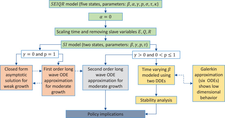
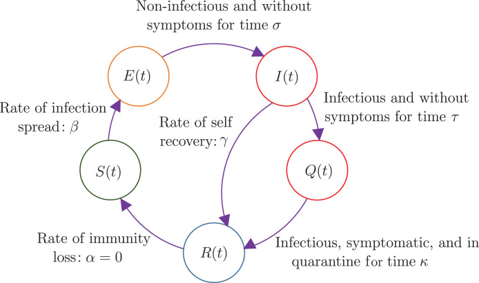
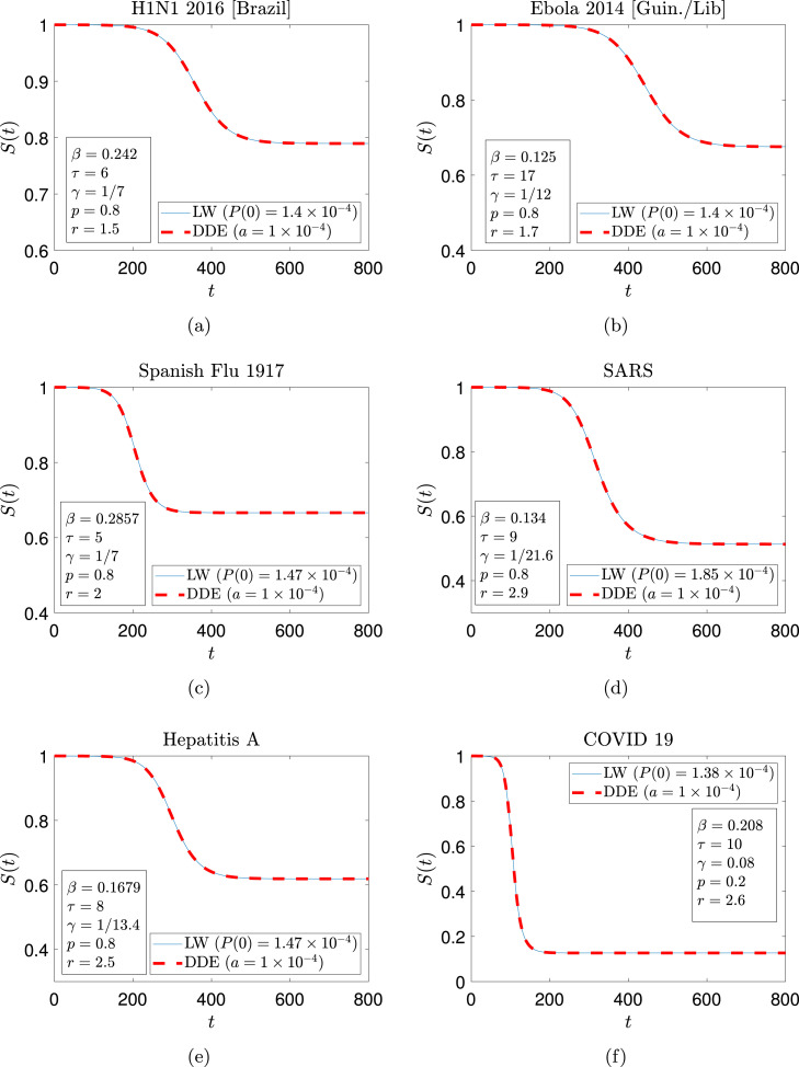
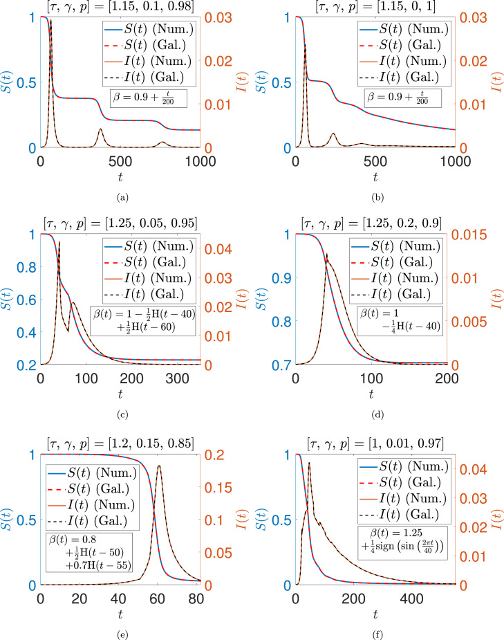
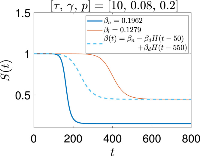
We study an SEIQR (Susceptible-Exposed-Infectious-Quarantined-Recovered) model due to Young et al. (2019) for an infectious disease, with time delays for latency and an asymptomatic phase. For fast pandemics where nobody has prior immunity and everyone has immunity after recovery, the SEIQR model decouples into two nonlinear delay differential equations (DDEs) with five parameters. One parameter is set to unity by scaling time. The simple subcase of perfect quarantining and zero self-recovery before quarantine, with two free parameters, is examined first. The method of multiple scales yields a hyperbolic tangent solution; and a long-wave (short delay) approximation yields a first order ordinary differential equation (ODE). With imperfect quarantining and nonzero self-recovery, the long-wave approximation is a second order ODE. These three approximations each capture the full outbreak, from infinitesimal initiation to final saturation. Low-dimensional dynamics in the DDEs is demonstrated using a six state non-delayed reduced order model obtained by Galerkin projection. Numerical solutions from the reduced order model match the DDE over a range of parameter choices and initial conditions. Finally, stability analysis and numerics show how a well executed temporary phase of social distancing can reduce the total number of people affected. The reduction can be by as much as half for a weak pandemic, and is smaller but still substantial for stronger pandemics. An explicit formula for the greatest possible reduction is given.

Keywords: COVID-19; Epidemic; Long-wave solution; Multiple scales; Social distancing.

Fig. 1

Flow chart showing the overview of the paper.

Fig. 2

The SEIQR model with delays. Healthy individuals $S\left(t\right)$ are infected with rate constant $\beta$. Infected individuals $E\left(t\right)$ remain asymptomatic and non-infectious for a time duration $\sigma$. Subsequently, these individuals become infectious and enter population $I\left(t\right)$, but remain asymptomatic for a time duration $\tau$. Upon showing symptoms, they enter population $Q\left(t\right)$ and are quarantined with probability $p$ for a time $\kappa$, beyond which they infect nobody. Some infectious asymptomatic individuals may become non-infectious on their own, with rate $\gamma$. After quarantine, the cured population $R\left(t\right)$ could in principle lose immunity at a small rate $\alpha$, but we take $\alpha =0$ for a fast-spreading pandemic.

Fig. 3

Two solutions each for (a) $\beta \tau =0.8<1$ and (b) $\beta \tau =1.2>1$. The initial function used for integrating Eq. (18) was $P\left(t\right)=a\left(1+\frac{t}{1+\tau }\right),t\le 0$. The two solutions in (b) are relatively time-shifted because the underlying system is autonomous, and one solution grows from smaller initial values; see main text for further discussion.

Fig. 4

Two solutions for (a) $\beta \tau =1.2>1$ and (b) $\beta \tau =2>1$. The parameters $\beta$ and $\tau$ are individually varied. The initial function used for integrating Eq. (18) was $P\left(t\right)=1\times 10^{-4}\left(1+\frac{t}{1+\tau }\right),t\le 0$.

Fig. 5

Comparison between numerical solution and asymptotic (method of multiple scales, or MMS) solution for (a) $\beta =1$, $\tau =1.025$, $a=1\times 10^{-5}$ (numerical) and $c_1=310$ (MMS); (b) $\beta =1$, $\tau =1.05$, $a=1\times 10^{-5}$ (numerical) and $c_1=200.5$ (MMS). The initial condition used for integrating Eq. (18) is $P\left(t\right)=a\left(1+\frac{t}{1+\tau }\right),t\le 0$. The arbitrary time-shift $c_1$ of the multiple scales solution (Eq. (47)) is chosen here to obtain a good visual match.

Fig. 6

Comparison between numerical, multiple scales (MMS), and long-wave solutions for (a) $\beta =1$, $\tau =1.15$, $a=1\times 10^{-5}$ (numerical), $c_1=93$ (MMS), and $P\left(0\right)=0.87\times 10^{-4}$ (long-wave); (b) $\beta =1$, $\tau =1.25$, $a=1\times 10^{-5}$ (numerical), $c_1=66$ (MMS), and $P\left(0\right)=0.78\times 10^{-4}$ (long-wave). The initial condition used for integrating Eq. (18) is $P\left(t\right)=a\left(1+\frac{t}{1+\tau }\right),t\le 0$. The initial condition $P\left(0\right)$ is used to integrate the long-wave equation (59). The coefficient $c_1$ is used in the multiple scales solution (see Eq. (47)).

Fig. 7

Comparison between numerical solution of Eq. (15) and long-wave solutions for (a) $\beta =1$, $\tau =1.25$, $\gamma =0.1$, $p=0.98$, $a=1\times 10^{-5}$ (DDE), and $P\left(0\right)=0.55\times 10^{-4}$ (long-wave); (b) Phase portrait of the long wave Eq. (62), the red thick line is the solution of Eq. (15).

Fig. 8

Comparison between numerical solution (of the DDE) and long-wave solutions for parameter sets corresponding to six different diseases (a) H1N1 (Brazil)  (b) Ebola  (c) Spanish Flu 1917  (d) SARS  (e) Hepatitis A , and (f) COVID-19 , . Initial conditions and other parameter values used to generate the results are shown in each figure separately.

Fig. 9

Comparison between numerical and Galerkin solutions for various parameters. $H(t-c)=1$ if $t>c$, and is zero otherwise. Initial functions used for Eqs. (70), (71) are $S\left(t\right)=1-10^{-5}\left(1+\frac{t}{1+\tau }\right),t\le 0$ and $I\left(t\right)=10^{-5}\left(1+\frac{t}{1+\tau }\right),t\le 0$. Initial conditions for Eqs. (72)–(77) are fitted by Galerkin projection (see the appendix).

Fig. 10

Fraction of susceptible population with $\beta \left(t\right)={\beta }_n=0.1962$, $\beta \left(t\right)={\beta }_l=0.1279$, and $\beta \left(t\right)={\beta }_n-{\beta }_{d}H(t-55)+{\beta }_{d}H(t-550)$. The parameters used for the generating the results are $\gamma =0.08$, $p=0.2$, and $\tau =10$. Here ${\beta }_d={\beta }_n-{\beta }_l$.

References

-
- Vynnycky E., White R. Oxford University Press; Oxford: 2010. An Introduction To Infectious Disease Modelling.
- Capasso V. Mathematical Structures of Epidemic Systems. vol. 97. Springer-Verlag; Berlin: 1993. (Lecture Notes in Biomath). - DOI
- Kermack W.O., McKendrick A.G. A contribution to the mathematical theory of epidemics. Proc. R. Soc. Lond. Ser. A Math. Phys. Eng. Sci. 1927;115:700–721. doi: 10.1098/rspa.1927.0118. - DOI
- Brauer F., Castillo-Chavez C. Mathematical Models in Population Biology and Epidemiology. Springer-Verlag; New York: 2001. (Texts in Applied Mathematics, vol. 2). - DOI
- Hethcote H.W. Applied Mathematical Ecology. Springer-Verlag; Berlin: 1989. Three basic epidemiological models; pp. 119–144. - DOI
LinkOut - more resources
Full Text Sources