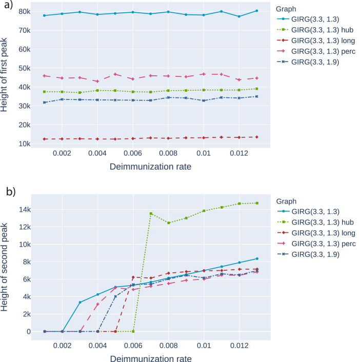
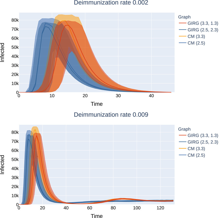
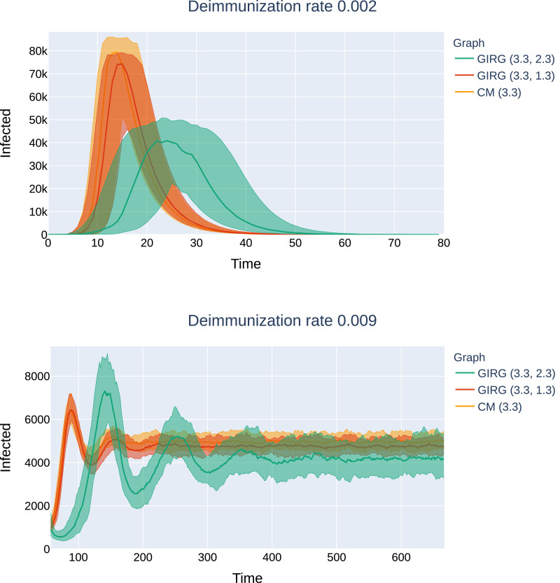
Not all interventions are equal for the height of the second peak

Abstract

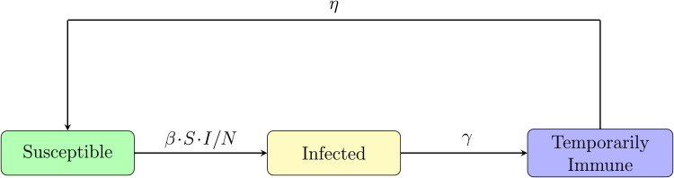
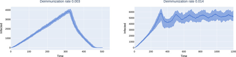
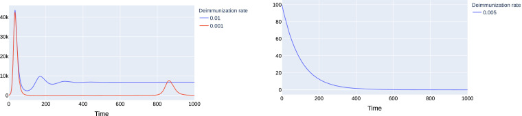
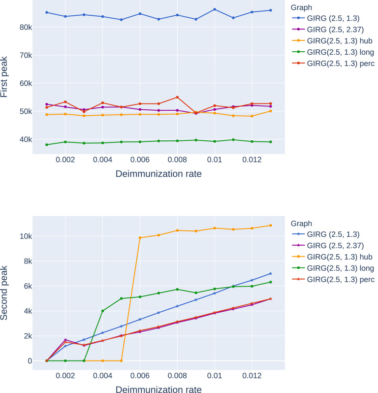
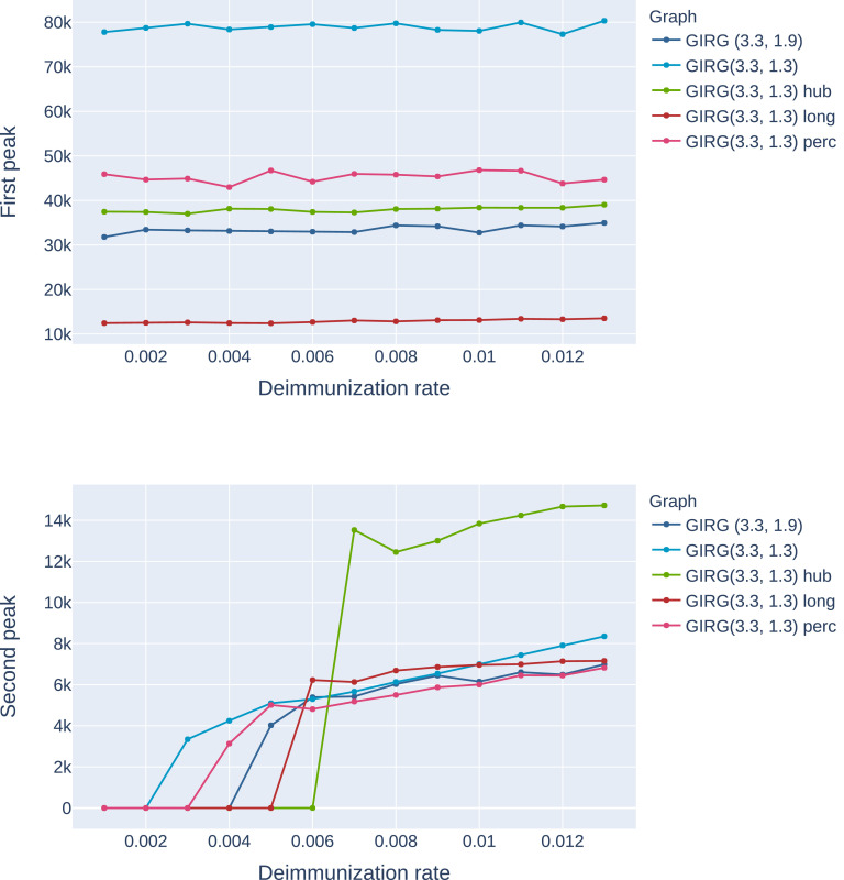
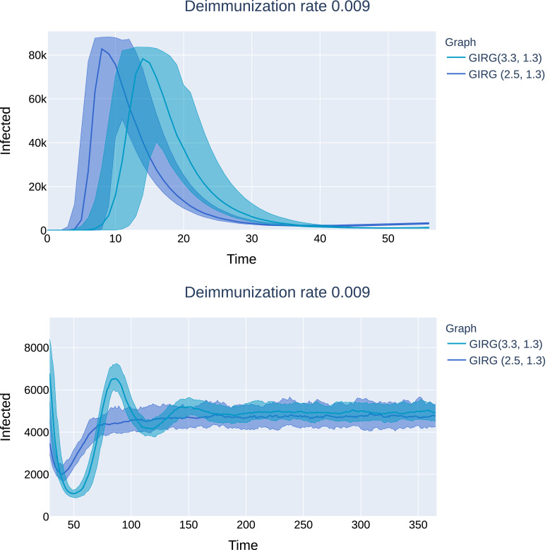
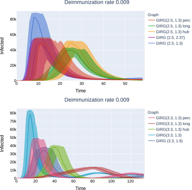
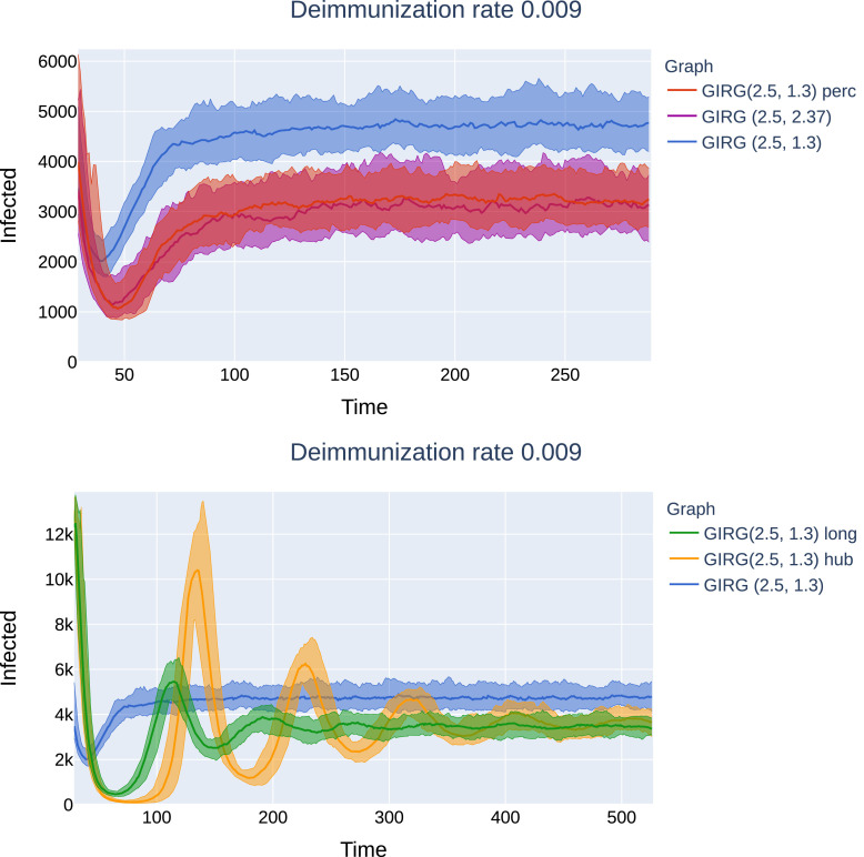
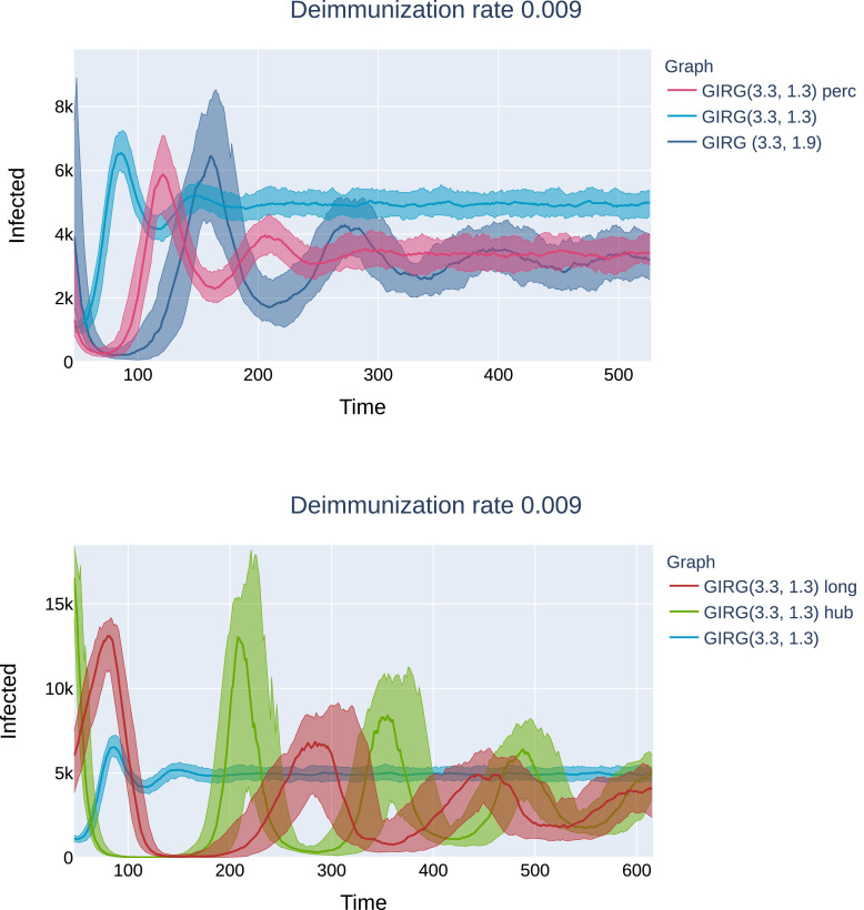
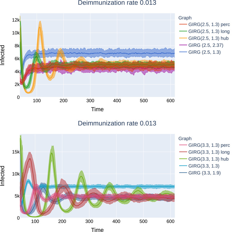
In this paper we conduct a simulation study of the spread of an epidemic like COVID-19 with temporary immunity on finite spatial and non-spatial network models. In particular, we assume that an epidemic spreads stochastically on a scale-free network and that each infected individual in the network gains a temporary immunity after its infectious period is over. After the temporary immunity period is over, the individual becomes susceptible to the virus again. When the underlying contact network is embedded in Euclidean geometry, we model three different intervention strategies that aim to control the spread of the epidemic: social distancing, restrictions on travel, and restrictions on maximal number of social contacts per node. Our first finding is that on a finite network, a long enough average immunity period leads to extinction of the pandemic after the first peak, analogous to the concept of "herd immunity". For each model, there is a critical average immunity duration L_c above which this happens. Our second finding is that all three interventions manage to flatten the first peak (the travel restrictions most efficiently), as well as decrease the critical immunity duration L_c , but elongate the epidemic. However, when the average immunity duration L is shorter than L_c , the price for the flattened first peak is often a high second peak: for limiting the maximal number of contacts, the second peak can be as high as 1/3 of the first peak, and twice as high as it would be without intervention. Thirdly, interventions introduce oscillations into the system and the time to reach equilibrium is, for almost all scenarios, much longer. We conclude that network-based epidemic models can show a variety of behaviors that are not captured by the continuous compartmental models.

Keywords: Agent-based epidemic modeling; COVID-19 Intervention strategies; Spatio-temporal network analysis; Temporary immunity; Theoretical epidemiology.

Fig. 1

Visualization of the change in the underlying contact network under interventions for Scenario 3 (see Fig. 26 below). By (w) and (s) we denote the weak and strong travel restrictions, respectively.

Fig. 2

Schematic diagram of node states and their transition probabilities. A susceptible node u may only become infected when it has at least one infected neighbor. Each of the infected neighbors infects u with probability β, independently, in each step.

Fig. 3

A comparison of the probability of phase 2M on eight different networks with the same average degree 8 and number of nodes $N=160000,$as a function of the η. Probabilities were computed using a 100 runs for all parameter values (η) and models, with $\beta =0.225,\gamma =0.2$. Legend: CM, GIRG: Scenarios 2 and 3, with different parameters and Grid: Scenario 1. For all networks we see a sharp transition at a critical value of ηwhere the system moves from phase 2P (single peak followed by extinction) to 2M (survival with multiple peaks) with overwhelming probability.

Fig. 4

The effect of interventions on the first and second peak, as a function of η (the inverse of the average immunity period). Abbreviations in the legend: ‘hub’: limiting maximal node degree, ‘long’: strong restriction on travel, ‘perc’: social distancing. The first entry is increasing α, a weak restriction on travel. GIRG(3.3,1.3) is the original network. We see that the height of the first peak is insensitive to the duration of immunity, and that cutting long edges is most effective in reducing the first peak. For the second peak, limiting node degree pushes the critical η for appearance of the second peak from 0.002 to 0.006, however, above that the second peak is twice as high as for other interventions. See also Fig. 21, Fig. 22.

Fig. 5

Schematic diagram of states and their transition rates in the continuous compartmental model. Infected individuals make contact at rate β to randomly chosen individuals, as a result, the number of susceptibles increases at rate β · S · I/N. This is a mean-field approximation of the graph model in Section 1.1, see Fig. 2.

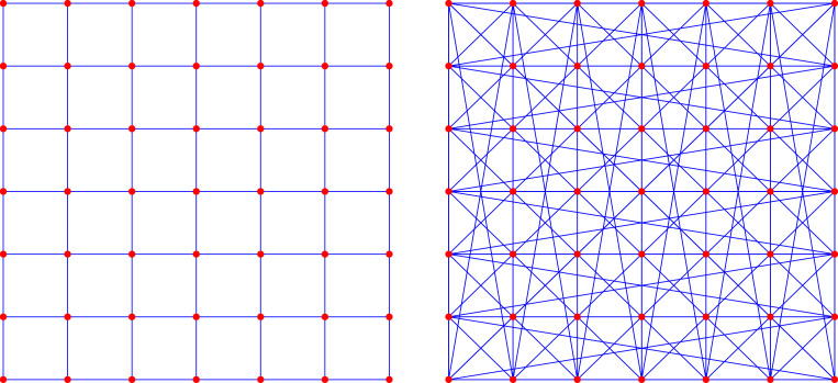
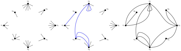
Fig. 6

Left: The two dimensional torus ${\mathbb{Z}}_7^2$on $N=49$nodes. Each node has four neighbors. Right: The modified two dimensional torus ${\tilde{\mathbb{Z}}}_7^2$on $N=49$nodes. Each node has 8 neighbors. The nodes in the bottom row are also connected to the nodes in the top row, and the nodes in the very left column are also connected to the nodes in the very right column.

Fig. 7

The algorithm producing the configuration model. Left: First, for each node in the network we prescribe its degree and draw it as half-edges. Middle: Then, we match half-edges randomly to form edges (connections). This may be done in a sequential way, by always choosing a uniform pair from the remaining half-edges. Here, an intermediate stage is shown when there are five edges formed. Right: All half-edges are matched. The output is a random graph called the configuration model.

Fig. 8

Two examples of the configuration model. The $N=200$nodes have average degree 4, with power-law degree distribution, with exponent $\tau =2.9$(left) and $\tau =3.3$(right).

Fig. 9

Two examples of Geometric Inhomogeneous Random Graphs (GIRGs). The $N=1000$nodes are placed randomly into a square of area N. Each node draws a random fitness from a power law distribution with exponent $\tau =2.95$(left) and $\tau =3.3$(right). We used the same location for nodes and the same underlying uniform variables to simulate fitnesses in both cases: for a uniform variable $U_v\in [0,1],$we set the fitness of node $v$to $W_v^{\left(2.95\right)}:=U_v^{-1/1.95}$on the left, while $W_v^{\left(3.3\right)}:=U_v^{-1/2.3}$on the right. Each pair of nodes with positions x₁, x₂ and weights $w_1,w_2,$respectively, is connected with probability $p^{\left(\tau \right)}=0.5(1\wedge 0.2(w_1^{\left(\tau \right)}{w}_2^{\left(\tau \right)}|x_1-x_2|{}^{-d}\left){}^{\alpha }\right),$where $\alpha =2.5$. Connections are again generated in a coupled way, using the same set of uniform variables for the two pictures, thresholded at p^(2.95)and p^(3.3), respectively.

Fig. 10

A comparison of survival probability of S-I-T-S on eight different networks with the same average degree, as a function of the η, the rate of losing immunisation. Survival probabilities were computed using a 100 runs for all parameter values (η) and models. The infection and healing rates $\beta =0.225,\gamma =0.2$for all cases. CM: the configuration model with $\tau =2.5,3.3,$GIRG: GIRG power-law fitnesses with $(\tau ,\alpha )=(2.5,2.3),(3.3,1.3),(3.3,2.3),$and Grid: the modified lattice ${\tilde{\mathbb{Z}}}^2$. All networks have the same number of $N=160000$nodes, and the same average degree $\mathbb{E}\left[\mathrm{deg}\right(u\left)\right]=8$. For all networks we see a sharp transition at a critical value of ηwhere the system moves from phase 2P (single peak followed by extinction) to 2M (survival with multiple peaks) with overwhelming probability.

Fig. 11

No intervention. Mean field network vs spatial scale-free networks with many long-range edges. A comparison of the number of infected on the configuration model versus GIRG with matching parameters. The continuous line shows the median of infected individuals, the shaded area is covers 95% of all runs for which the number of infected nodes was positive. Each model has average degree 8. Observe that the epidemic curve of configuration model with $\tau =2.5$(CM(2.5), dark blue) matches that of GIRG with $(\tau ,\alpha )=(2.5,2.3)$(GIRG(2.5,2.3), light blue), while the epidemic curve of the configuration model with $\tau =3.3$(CM(3.3), yellow) matches that of that of GIRG with $(\tau ,\alpha )=(3.3,1.3)$(GIRG(3.3,1.3), red) Top: $\eta =0.002$(500 days immunity), a single peak can be observed. Bottom: $\eta =0.009$(111 days immunity), many peaks can be observed. (For interpretation of the references to colour in this figure legend, the reader is referred to the web version of this article.)

Fig. 12

No intervention: The effect of geometry. Each model has average degree 8, and power-law exponent $\tau =3.3$. We see that there is only a match between the mean field network configuration model (CM) when α < 2, hence, there are many long-range connections in the network. The epidemic curve of configuration model with $\tau =3.3$(CM(3.3), orange) matches that of GIRG with $(\tau ,\alpha )=(3.3,1.3)$(GIRG(3.3,1.3), red). When α is increased to 2.3 (GIRG(3.3,2.3), green). This effects the first peak of epidemic curve to flatten, its magnitude is shrunk by almost 40%, even though the average degree is tuned to remain the same. Top:$\eta =0.002$(500 days immunity) On all three models, a single peak can be observed, and all runs die out within 70 days. Bottom: $\eta =0.009,$the first peak has the same height as on to the top picture and is not shown. Without intervention (GIRG(3.3,1.3)), the second and further peaks of the epidemic behave similarly to the mean-field network (CM(3.3)). With intervention, (GIRG(3.3,2.3)), both the oscillation period as well as its amplitude are higher, but the average stationary proportion of infected nodes is lower. (For interpretation of the references to colour in this figure legend, the reader is referred to the web version of this article.)

Fig. 13

A comparison of the number of infected on the torus ${\tilde{Z}}_n^2$with $n=400,$in total $N=160000$nodes, $\gamma =0.2,$$\beta =0.225$for two values of η, see in subfigure captions. The continuous curve shows the median, the shaded area 95% of all runs of all runs for which the number of infected nodes was positive.

Fig. 14

Solutions of the ODE when $N=160000,\gamma =0.14$with 100 initially infected nodes. The infection almost seemingly disappears from the system before the second peak appears when $\eta =0.001$. The infection does not turn into a pandemic when β < γ.

Fig. 15

Visualization of the change in the underlying contact network under interventions. The network on the top left is similar to G₁: a GIRG with $(\tau ,\alpha )=(2.5,1.3),$average degree 4.8 on $N=1000$nodes. All interventions result in an average degree  ≈ 2.6.

Fig. 16

Visualization of the change in the underlying contact network under interventions. The network on the top left is similar to G₂: a GIRG with $(\tau ,\alpha )=(3.3,1.3),$average degree 4.8 on $N=1000$nodes. All interventions result in an average degree  ≈ 2.6, just like on Fig. 15, even though the pictures here look much more sparse.

Fig. 17

Visualization of the initial 19 days on G₁ under interventions. The network on the top left is G₁, a GIRG with $(\tau ,\alpha )=(2.5,1.3)$and average degree 9.6 on $N=160000$nodes. All interventions result in an average degree 5.7. The darker the color, the earlier the infection. We chose typical runs to illustrate the effect of interventions.

Fig. 18

Visualization of the initial 19 days on G₂ under several intervention measures. The network on the left is G₂, a GIRG with $(\tau ,\alpha )=(3.3,1.3)$and average degree 8.7 on $N=160000$nodes. All interventions result in an average degree 4.9. The darker the color, the earlier the infection. Color scaling is the same as on Fig. 17.

Fig. 19

The effect of interventions: the long-survival probabilities (phase 2M) are decreasing significantly under each intervention strategy. The four interventions are: (A) social distancing, denoted as ”perc”, (B) limiting maximal degree, denoted as ”hub”, (Ch) a hard no-travel rule, denoted as ”long” on the legend, and (Cw) a weak no-travel rule: increasing α. We see that in all interventions, the long-survival probabilities are below the original curve. The threshold η is lowest for percolation and highest for limiting the maximal degree, while truncating long-edges and increasing α in the network both show an interesting non-monotonous survival probability curve. Top: The initial network is G₁, a GIRG with $(\tau ,\alpha )=(2.5,1.3),$and $\mathbb{E}\left[\mathrm{deg}\right(u\left)\right]=9.6$. Bottom:The initial network is G₂, a GIRG with $(\tau ,\alpha )=(3.3,1.3),$and $\mathbb{E}\left[\mathrm{deg}\right(u\left)\right]=8.7$.

Fig. 20

Monotonicity of survival probabilities as a function of η. For the graph $G_2^{\alpha },$a GIRG(3.3, 1.9) (weak no-travel rule), we have tested the monotonicity of the survival probability curve, by increasing the number of runs to 500 for each value of η. The curve appears to be monotonous, with a sharp threshold near η_c ≈ 0.007.

Fig. 21

The effect of interventions on the first and second peak on G₁, as a function of η (the inverse of the average immunity period). Abbreviations in the legend: ‘hub’: limiting maximal node degree, ‘long’: cutting long edges, ‘perc’: social distancing. The first entry is increasing α. GIRG(2.3,1.3) is the original network. We see that the height of the first peak is insensitive to the immunity duration, and that cutting long edges is most effective in reducing the first peak. For the second peak, limiting node degree pushes the critical η for appearance of the second peak from basically 0 to 0.005, however, above that the second peak is twice as high as for other interventions. Cutting long-edges also has a similar effect, although to a lesser extent. See also Figure 4. Star indicates that there is no second peak, and the height we see is the height of the equilibrium, see the top figure on Fig. 25.

Fig. 22

The effect of interventions on the first and second peak on G₂, as a function of η (the inverse of the average immunity period). Abbreviations in the legend: ‘hub’: limiting maximal node degree, ‘long’: cutting long edges, ‘perc’: social distancing. The first entry is increasing α. GIRG(3.3,1.3) is the original network. We see that the height of the first peak is insensitive to the immunity duration, and that cutting long edges is most effective in reducing the first peak. For the second peak, limiting node degree pushes the critical η for appearance of the second peak from 0.002 to 0.006, however, above that the second peak is twice as high as for other interventions. See also Figure 21.

Fig. 23

No intervention: the epidemic curves for the networks G₁, G₂ on which we apply the intervention methods. G₁ is a GIRG with $(\tau ,\alpha )=(2.5,1.3)$and average degree 9.6, while G₂ is a GIRG with $(\tau ,\alpha )=(2.5,1.3)$and average degree 8.7. Top: The first peak of the epidemic. Bottom: The second peak and stabilization of the number of infected. The average height and location of the first peak is ${\overline{H}}_1\left(G_1\right)=82785$on day 8 for G₁, while it is ${\overline{H}}_1\left(G_2\right)=78263$on day 14 for GIRG with $(\tau ,\alpha )=(3.3,1.3)$. On G₂, we see a second peak at day 79 of average height ${\overline{H}}_2\left(G_2\right)=6538,$and the equilibrium number of infected $\overline{E}\left(G_2\right)\approx 5000\pm 100$. The equilibrium number of infected $\overline{E}\left(G_1\right)\approx 4700\pm 100$is reached without a second peak on G₁.

Fig. 24

The first peak under interventions. Top: The effect of interventions on G₁: Social distancing (“GIRG(2.5, 1.3) perc”), the hard no travel rule (“GIRG(2.5, 1.3) long”), limiting the maximal number of contact (“GIRG(2.5, 1.3) hub”), and the weak no-travel rule (“GIRG(2.5, 2.37)”). The first peak disappears before day 60 in all cases. The curves for the weak no-travel rule and social distancing are almost identical. Bottom: The effect of interventions on G₁: Social distancing (“GIRG(3.3, 1.3) perc”), the hard no travel rule (“GIRG(3.3, 1.3) long”), limiting the maximal number of contact (“GIRG(3.3, 1.3) hub”), and the weak no-travel rule (“GIRG(3.3, 1.9)”). The hard no travel rule is most effective in flattening the curve: both in its height as well as the day of the peak.

Fig. 25

Later effects of interventions on G₁: Top: Social distancing (“GIRG(2.5, 1.3) perc”), as well as the weak no-travel rule (“GIRG(2.5, 2.37)”). No second peak can be observed, just like on the original network. Bottom: Limiting the maximal number of contact (“GIRG(2.5, 1.3) hub”), and the hard no travel rule (“GIRG(2.5, 1.3) long”’): second and further peaks are periodically present, with decreasing magnitude and period roughly the average immunity duration. G₁ is a GIRG with $(\tau ,\alpha )=(2.5,1.3)$and average degree 9.6 on $N=160000$nodes. All networks after intervention have average degree  ≈ 4.9.

Fig. 26

Later effects of interventions on G₂: Top: Social distancing (“GIRG(3.3, 1.3) perc”), as well as the weak no-travel rule (“GIRG(3.3, 1.9)”) compared to the original network (“GIRG(3.3, 1.3)”). Second and further peaks are present, equilibrium is reached within 600 days. Bottom: Limiting the maximal number of contact (“GIRG(3.3, 1.3) hub”), and the hard no travel rule (“GIRG(3.3, 1.3) long”’): second and further peaks are more profound, equilibrium is only reached around 1200 days. G₂ is a GIRG with $(\tau ,\alpha )=(3.3,1.3)$and average degree 8.7 on $N=160000$nodes. All networks after intervention have average degree  ≈ 4.7. The first peak can be seen on Fig. 24. The first peak of the red curve (corresponding to truncating long edges) is the first peak of the epidemic. (For interpretation of the references to colour in this figure legend, the reader is referred to the web version of this article.)

Fig. 27

Later effects of interventions on G₁, G₂, for $\eta =0.013$: Top: G₁and all interventions. Bottom G₂ and all interventions. The curves are qualitatively similar to $\eta =0.009,$the period between second and further peaks differ from those on Figs. 25 and 25. The first peak is not affected by the change of η (below 2% change in height, that could be also due to statistical error margins, so we omit to plot it. The first peak of the red curve (corresponding to truncating long edges) is the first peak of the epidemic. (For interpretation of the references to colour in this figure legend, the reader is referred to the web version of this article.)

References

-
- Albert R., Barabási A.L. Statistical mechanics of complex networks. Rev Mod Phys. 2002;74(1):47.
- Barabási A., Albert R. Emergence of scaling in random networks. Science (New York, NY) 1999;286(5439) - PubMed
- Barbour A., Reinert G. Approximating the epidemic curve. Electronic Journal Of Probability. 2013;18:1–30.
- Berger N., Borgs C., Chayes J.T., Saberi A. Proceedings of the sixteenth annual ACM-SIAM symposium on Discrete algorithms. Society for Industrial and Applied Mathematics; 2005. On the spread of viruses on the internet; pp. 301–310.
LinkOut - more resources
Full Text Sources