Integrating genotypes and phenotypes improves long-term forecasts of seasonal influenza A/H3N2 evolution

Abstract

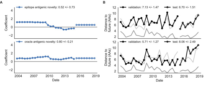
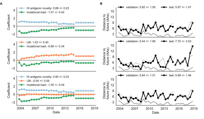
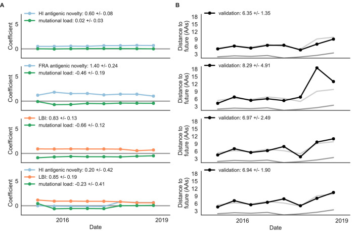
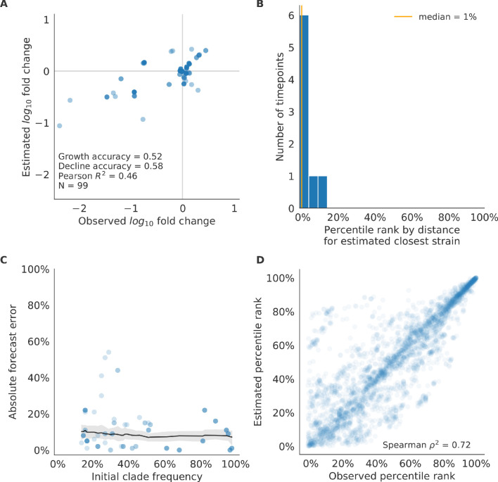
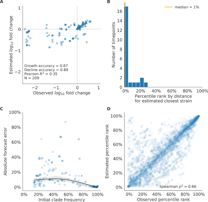
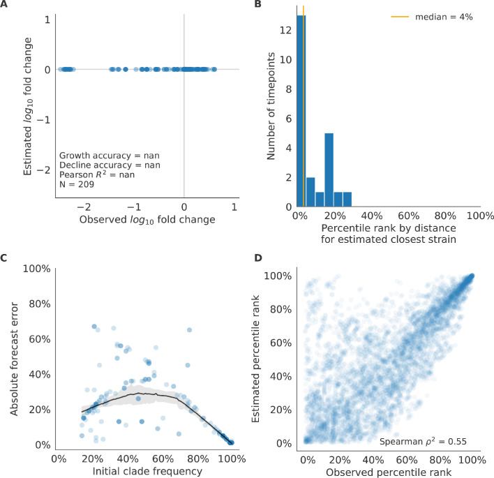
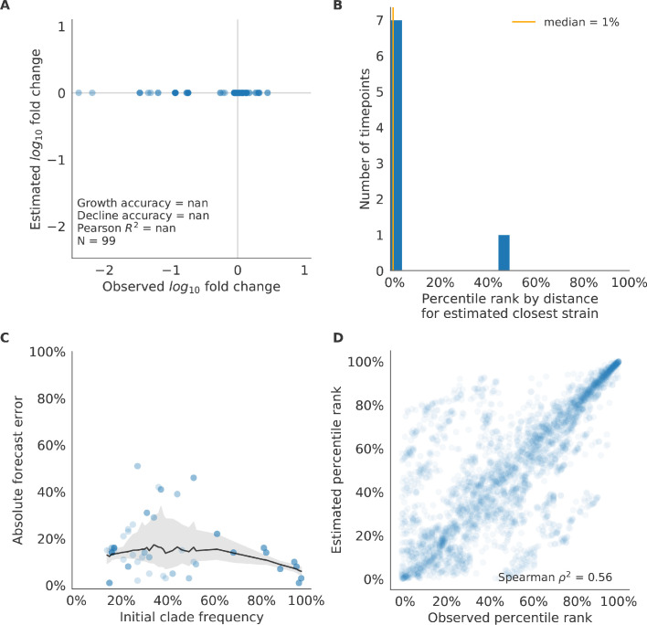
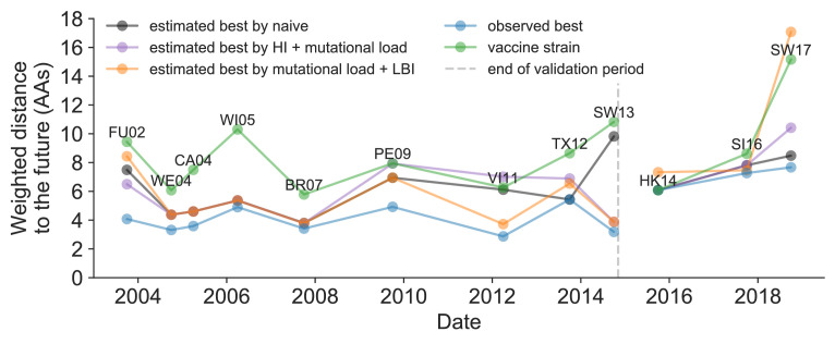
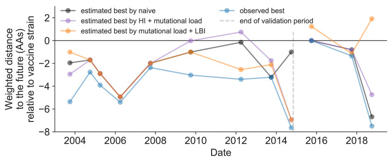
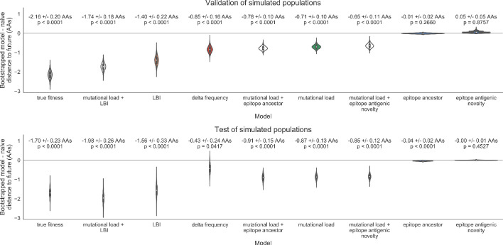
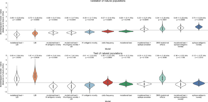
Seasonal influenza virus A/H3N2 is a major cause of death globally. Vaccination remains the most effective preventative. Rapid mutation of hemagglutinin allows viruses to escape adaptive immunity. This antigenic drift necessitates regular vaccine updates. Effective vaccine strains need to represent H3N2 populations circulating one year after strain selection. Experts select strains based on experimental measurements of antigenic drift and predictions made by models from hemagglutinin sequences. We developed a novel influenza forecasting framework that integrates phenotypic measures of antigenic drift and functional constraint with previously published sequence-only fitness estimates. Forecasts informed by phenotypic measures of antigenic drift consistently outperformed previous sequence-only estimates, while sequence-only estimates of functional constraint surpassed more comprehensive experimentally-informed estimates. Importantly, the best models integrated estimates of both functional constraint and either antigenic drift phenotypes or recent population growth.

Keywords: antigenic drift; evolution; evolutionary biology; infectious disease; influenza; microbiology; phenotypes; prediction; virus.

Figure 1.. Schematic representation of the fitness model for simulated H3N2-like populations wherein the fitness of strains at timepoint t determines the estimated frequency of strains with similar sequences one year in the future at timepoint u.

Strains are colored by their amino acid sequence composition such that genetically similar strains have similar colors (Materials and methods). (A) Strains at timepoint t, $\mathbf{𝐱}(t)$, are shown in their phylogenetic context and sized by their frequency at that timepoint. The estimated future population at timepoint u, $\widehat{\mathbf{𝐱}}(u)$, is projected to the right with strains scaled in size by their projected frequency based on the known fitness of each simulated strain. (B) The frequency trajectories of strains at timepoint t to u represent the predicted the growth of the dark blue strains to the detriment of the pink strains. (C) Strains at timepoint u, $\mathbf{𝐱}(u)$, are shown in the corresponding phylogeny for that timepoint and scaled by their frequency at that time. (D) The observed frequency trajectories of strains at timepoint u broadly recapitulate the model’s forecasts while also revealing increased diversity of sequences at the future timepoint that the model could not anticipate, e.g. the emergence of the light blue cluster from within the successful dark blue cluster. Model coefficients minimize the earth mover’s distance between amino acid sequences in the observed, $\mathbf{𝐱}(u)$, and estimated, $\widehat{\mathbf{𝐱}}(u)$, future populations across all training windows.

Figure 2.. Time-series cross-validation scheme for simulated populations.

Models were trained in six-year sliding windows (gray lines) and validated on out-of-sample data from validation timepoints (filled circles). Validation results from 30 years of data were used to iteratively tune model hyperparameters. After fixing hyperparameters, model coefficients were fixed at the mean values across all training windows. Fixed coefficients were applied to 9 years of new out-of-sample test data (open circles) to estimate true forecast errors.

Figure 3.. Phylogeny of H3N2-like HA sequences sampled between the 24th and 30th years of simulated evolution.

The phylogenetic structure and rate of accumulated epitope and non-epitope mutations match patterns observed in phylogenies of natural sequences. Sample dates were annotated as the generation in the simulation divided by 200 and added to 2000, to acquire realistic date ranges that were compatible with our modeling machinery.

Figure 4.. Simulated population model coefficients and distances between projected and observed future populations as measured in amino acids (AAs).

(A) Coefficients are shown per validation timepoint (solid circles, N = 33) with the mean ± standard deviation in the top-left corner. For model testing, coefficients were fixed to their mean values from training/validation and applied to out-of-sample test data (open circles, N = 18). (B) Distances between projected and observed populations are shown per validation timepoint (solid black circles) or test timepoint (open black circles). The mean ± standard deviation of distances per validation timepoint are shown in the top-left of each panel. Corresponding values per test timepoint are in the top-right. The naive model’s distances to the future for validation and test timepoints (light gray) were 8.97 ± 1.35 AAs and 9.07 ± 1.70 AAs, respectively. The corresponding lower bounds on the estimated distance to the future (dark gray) were 4.57 ± 0.61 AAs and 4.85 ± 0.82 AAs. Source data are in Table 4—source data 1 and 2.

Figure 5.. Simulated population model coefficients and distances to the future for individual biologically-informed fitness metrics and the best composite model.

(A) Coefficients and (B) distances are shown per validation and test timepoint as in Figure 4. Source data are in Table 4—source data 1 and 2.

Figure 5—figure supplement 1.. Composite model coefficients and distances to the future for models fit to simulated populations.

(A) Coefficients and (B) distances are shown per validation timepoint and test timepoint as in Figure 4. Source data are in Table 4—source data 1 and 2.

Figure 6.. Test of best model for simulated populations (true fitness) using 9 years (18 timepoints) of previously unobserved test data and fixed model coefficients.

These timepoints correspond to the open circles in Figure 2. (A) The correlation of log estimated clade frequency fold change, ${\log }_{10}\frac{\widehat{x}(t+\mathrm{\Delta }t)}{x(t)}$, and log observed clade frequency fold change, ${\log }_{10}\frac{x(t+\mathrm{\Delta }t)}{x(t)}$, shows the model’s ability to capture clade-level dynamics without explicitly optimizing for clade frequency targets. (B) The rank of the estimated closest strain based on its distance to the future in the best model was in the top 20th percentile for 89% of 18 timepoints, confirming that the model makes a good choice when forced to select a single representative strain for the future population. (C) Absolute forecast error for clades shown in A by their initial frequency with a mean LOESS fit (solid black line) and 95% confidence intervals (gray shading) based on 100 bootstraps. (D) The correlation of all strains at all timepoints by the percentile rank of their observed and estimated distances to the future. The corresponding results for the naive model are shown in Figure 6—figure supplement 3.

Figure 6—figure supplement 1.. Validation of best model for simulated populations of H3N2-like viruses.

Validation of best model for simulated populations of H3N2-like viruses for 33 timepoints. These timepoints correspond to the closed circles in Figure 2. (A) The correlation of estimated and observed clade frequency fold changes shows the model’s ability to capture clade-level dynamics without explicitly optimizing for clade frequency targets. (B) The rank of the estimated closest strain based on its distance to the future for 33 timepoints. The estimated closest strain was in the top 20th percentile of observed closest strains for 100% of timepoints, confirming that the model makes a good choice when forced to select a single representative strain for the future population. (C) Absolute forecast error for clades shown in A by their initial frequency with a mean LOESS fit (solid black line) and 95% confidence intervals (gray shading) based on 100 bootstraps. (D) The correlation of all strains at all timepoints by the percentile rank of their observed and estimated distances to the future. The corresponding results for the naive model are shown in Figure 6—figure supplement 2.

Figure 6—figure supplement 2.. Validation of naive model for simulated populations of H3N2-like viruses.

Validation of naive model for simulated populations of H3N2-like viruses for 33 timepoints. These timepoints correspond to the closed circles in Figure 2. Note that the naive model sets future frequencies to current frequencies such that there is no estimated fold change in frequencies for the first panel.

Figure 6—figure supplement 3.. Test of naive model for simulated populations of H3N2-like viruses.

Test of naive model for simulated populations of H3N2-like viruses for 18 timepoints. These timepoints correspond to the open circles in Figure 2. Note that the naive model sets future frequencies to current frequencies such that there is no estimated fold change in frequencies for the first panel.

Figure 7.. Time-series cross-validation scheme for natural populations.

Models were trained in six-year sliding windows (gray lines) and validated on out-of-sample data from validation timepoints (filled circles). Validation results from 25 years of data were used to iteratively tune model hyperparameters. After fixing hyperparameters, model coefficients were fixed at the mean values across all training windows. Fixed coefficients were applied to four years of new out-of-sample test data (open circles) to estimate true forecast errors.

Figure 8.. Natural population model coefficients and distances to the future for individual biologically-informed fitness metrics.

(A) Coefficients and (B) distances are shown per validation timepoint (N = 23) and test timepoint (N = 8) as in Figure 4. The naive model’s distance to the future (light gray) was 6.40 ± 1.36 AAs for validation timepoints and 6.82 ± 1.74 AAs for test timepoints. The corresponding lower bounds on the estimated distance to the future (dark gray) were 2.60 ± 0.89 AAs and 2.28 ± 0.61 AAs. Source data are in Table 6—source data 1 and 2.

Figure 8—figure supplement 1.. Comparison of epitope-based models with knowledge of the future.

Model coefficients and distances to the future for antigenic novelty models fit to natural populations. (A) Coefficients and (B) distances are shown per validation timepoint and test timepoint as in Figure 4. The epitope antigenic novelty model relies on previously published epitope sites (Luksza and Lässig, 2014). The ‘oracle’ antigenic novelty model relies on sites of beneficial mutations that were manually identified from the entire training and validation time period (Methods). The improved performance of the ‘oracle’ model indicates that the sequence-based antigenic novelty metric can be effective when sites of beneficial mutations are known prior to forecasting. Source data are in Table 6—source data 1 and 2.

Figure 9.. Natural population model coefficients and distances to the future for composite fitness metrics.

(A) Coefficients and (B) distances are shown per validation timepoint (N = 23) and test timepoint (N = 8) as in Figure 4. Source data are in Table 6—source data 1 and 2.

Figure 9—figure supplement 1.. Composite models fit to most recent data from natural populations.

Model coefficients and distances to the future for best composite models and a FRA-based composite fit to recent data from natural populations as in Figure 4. (A) Coefficients and (B) distances are shown per test timepoint (N = 8). In contrast to the results for these models based on fixed coefficients from training/validation, these coefficients were learned for each six-year window prior to the corresponding test timepoint. The corresponding distances reflect the model’s performance with updated coefficients on what is effectively new validation data. The naive model’s distance to the future was 6.82 ± 1.74 AAs for these timepoints.

Figure 10.. Test of best model for natural populations of H3N2 viruses, the composite model of HI antigenic novelty and mutational load, across eight timepoints.

These timepoints correspond to the open circles in Figure 7. (A) The correlation of estimated and observed clade frequency fold changes shows the model’s ability to capture clade-level dynamics without explicitly optimizing for clade frequency targets. (B) The rank of the estimated closest strain based on its distance to the future for eight timepoints. The estimated closest strain was in the top 20th percentile of observed closest strains for 100% of timepoints. (C) Absolute forecast error for clades shown in A by their initial frequency with a mean LOESS fit (solid black line) and 95% confidence intervals (gray shading) based on 100 bootstraps. (D) The correlation of all strains at all timepoints by the percentile rank of their observed and estimated distances to the future. The corresponding results for the naive model are shown in Figure 10—figure supplement 3.

Figure 10—figure supplement 1.. Validation of best model for natural populations of H3N2 viruses.

Validation of best model for natural populations of H3N2 viruses for 23 timepoints using the composite model of mutational load and LBI. These timepoints correspond to the closed circles in Figure 7. (A) The correlation of estimated and observed clade frequency fold changes shows the model’s ability to capture clade-level dynamics without explicitly optimizing for clade frequency targets. (B) The rank of the estimated closest strain based on its distance to the future for 23 timepoints. The estimated closest strain was in the top 20th percentile of observed closest strains for 87% of timepoints, confirming that the model makes a good choice when forced to select a single representative strain for the future population. (C) Absolute forecast error for clades shown in A by their initial frequency with a mean LOESS fit (solid black line) and 95% confidence intervals (gray shading) based on 100 bootstraps. (D) The correlation of all strains at all timepoints by the percentile rank of their observed and estimated distances to the future. The corresponding results for the naive model are shown in Figure 10—figure supplement 2.

Figure 10—figure supplement 2.. Validation of naive model for natural populations of H3N2 viruses.

Validation of naive model for natural populations of H3N2 viruses for 23 timepoints. These timepoints correspond to the closed circles in Figure 7. Note that the naive model sets future frequencies to current frequencies such that there is no estimated fold change in frequencies for the first panel.

Figure 10—figure supplement 3.. Test of naive model for natural populations of H3N2 viruses.

Test of naive model for natural populations of H3N2 viruses for eight timepoints. These timepoints correspond to the open circles in Figure 7. Note that the naive model sets future frequencies to current frequencies such that there is no estimated fold change in frequencies for the first panel.

Figure 11.. Observed distance to natural H3N2 populations one year into the future for each vaccine strain (green) and the observed (blue) and estimated closest strains to the future by the mutational load and LBI model (orange), the HI antigenic novelty and mutational load model (purple), and the naive model (black).

Vaccine strains were assigned to the validation or test timepoint closest to the date they were selected by the WHO. The weighted distance to the future for each strain was calculated from their amino acid sequences and the frequencies and sequences of the corresponding population one year in the future. Vaccine strain names are abbreviated from A/Fujian/411/2002, A/Wellington/1/2004, A/California/7/2004, A/Wisconsin/67/2005, A/Brisbane/10/2007, A/Perth/16/2009, A/Victoria/361/2011, A/Texas/50/2012, A/Switzerland/9715293/2013, A/HongKong/4801/2014, A/Singapore/Infimh-16-0019/2016, and A/Switzerland/8060/2017. Source data are available in Figure 11—source data 1.

Figure 11—figure supplement 1.. Relative improvement of model selections over vaccine strains.

Relative distance to future H3N2 populations between vaccine strains and corresponding observed and estimated closest strains at each timepoint as in Figure 11. Strains with relative distances greater than zero were farther from the future than the selected vaccine strain, while strains below zero were closer to the future. Source data are available in Figure 11—source data 1.

Figure 12.. Snapshot of live forecasts on nextstrain.org from our best model (HI antigenic novelty and mutational load) for April 1, 2021.

The observed frequency trajectories for currently circulating clades are shown up to April 1, 2020. Our model forecasts growth of the clades 3c3.A and A1b/94N and decline of all other major clades.

Figure 13.. Snapshot of the last two years of seasonal influenza H3N2 evolution on nextstrain.org showing the estimated distance per strain to the future population.

Distance to the future is calculated for each strain as the Hamming distance of HA amino acid sequences to all other circulating strains weighted by the other strain’s projected frequencies under the best fitness model (HI antigenic novelty and mutational load).

Figure 14.. Bootstrap distributions of the mean difference of distances to the future between biologically-informed and naive models for simulated populations.

Empirical differences in distances to the future were sampled with replacement and mean values for each bootstrap sample were calculated across n = 10,000 bootstrap iterations. The horizontal gray line indicates a difference of zero between a given model and its corresponding naive model. Each model is annotated by the mean ± the standard deviation of the bootstrap distribution. Models are also annotated by the p-value representing the proportion of bootstrap samples with values less than zero (see Methods).

Figure 15.. Bootstrap distributions of the mean difference of distances to the future between biologically-informed and naive models for natural populations.

Empirical differences in distances to the future were sampled with replacement and mean values for each bootstrap sample were calculated across n = 10,000 bootstrap iterations. The horizontal gray line indicates a difference of zero between a given model and its corresponding naive model. Each model is annotated by the mean ± the standard deviation of the bootstrap distribution. Models are also annotated by the p-value representing the proportion of bootstrap samples with values less than zero (see Materials and methods).

Author response image 1.. Distribution of distances to the future by Hemisphere for the best natural model (HI antigenic novelty and mutational load) subtracted from the corresponding distance to the future for the naive model at the same timepoint.

References

1. Barrat-Charlaix P, Huddleston J, Bedford T, Neher RA. Limited predictability of amino acid substitutions in seasonal influenza viruses. bioRxiv. 2020 doi: 10.1101/2020.07.31.231100. - DOI - PMC - PubMed
1. Bedford T, Suchard MA, Lemey P, Dudas G, Gregory V, Hay AJ, McCauley JW, Russell CA, Smith DJ, Rambaut A. Integrating influenza antigenic dynamics with molecular evolution. eLife. 2014;3:e01914. doi: 10.7554/eLife.01914. - DOI - PMC - PubMed
1. Bedford T, Riley S, Barr IG, Broor S, Chadha M, Cox NJ, Daniels RS, Gunasekaran CP, Hurt AC, Kelso A, Klimov A, Lewis NS, Li X, McCauley JW, Odagiri T, Potdar V, Rambaut A, Shu Y, Skepner E, Smith DJ, Suchard MA, Tashiro M, Wang D, Xu X, Lemey P, Russell CA. Global circulation patterns of seasonal influenza viruses vary with antigenic drift. Nature. 2015;523:217–220. doi: 10.1038/nature14460. - DOI - PMC - PubMed
1. Belongia EA, Simpson MD, King JP, Sundaram ME, Kelley NS, Osterholm MT, McLean HQ. Variable influenza vaccine effectiveness by subtype: a systematic review and meta-analysis of test-negative design studies. The Lancet Infectious Diseases. 2016;16:942–951. doi: 10.1016/S1473-3099(16)00129-8. - DOI - PubMed
1. Bradski G. The OpenCV Library. 4.3.0Dr Dobb’s Journal of Software Tools. 2000 https://opencv.org/
Publication types