. 2020 Sep 7:9:e57443.
doi: 10.7554/eLife.57443.

A connectome and analysis of the adult Drosophila central brain

Louis K Scheffer #  1 C Shan Xu #  1 Michal Januszewski #  2 Zhiyuan Lu #  1   3 Shin-Ya Takemura #  1 Kenneth J Hayworth #  1 Gary B Huang #  1 Kazunori Shinomiya #  1 Jeremy Maitlin-Shepard  4 Stuart Berg  1 Jody Clements  1 Philip M Hubbard  1 William T Katz  1 Lowell Umayam  1 Ting Zhao  1 David Ackerman  1 Tim Blakely  2 John Bogovic  1 Tom Dolafi  1 Dagmar Kainmueller  1 Takashi Kawase  1 Khaled A Khairy  1 Laramie Leavitt  2 Peter H Li  2 Larry Lindsey  2 Nicole Neubarth  1 Donald J Olbris  1 Hideo Otsuna  1 Eric T Trautman  1 Masayoshi Ito  1   5 Alexander S Bates  6 Jens Goldammer  1   7 Tanya Wolff  1 Robert Svirskas  1 Philipp Schlegel  6 Erika Neace  1 Christopher J Knecht  1 Chelsea X Alvarado  1 Dennis A Bailey  1 Samantha Ballinger  1 Jolanta A Borycz  3 Brandon S Canino  1 Natasha Cheatham  1 Michael Cook  1 Marisa Dreher  1 Octave Duclos  1 Bryon Eubanks  1 Kelli Fairbanks  1 Samantha Finley  1 Nora Forknall  1 Audrey Francis  1 Gary Patrick Hopkins  1 Emily M Joyce  1 SungJin Kim  1 Nicole A Kirk  1 Julie Kovalyak  1 Shirley A Lauchie  1 Alanna Lohff  1 Charli Maldonado  1 Emily A Manley  1 Sari McLin  3 Caroline Mooney  1 Miatta Ndama  1 Omotara Ogundeyi  1 Nneoma Okeoma  1 Christopher Ordish  1 Nicholas Padilla  1 Christopher M Patrick  1 Tyler Paterson  1 Elliott E Phillips  1 Emily M Phillips  1 Neha Rampally  1 Caitlin Ribeiro  1 Madelaine K Robertson  3 Jon Thomson Rymer  1 Sean M Ryan  1 Megan Sammons  1 Anne K Scott  1 Ashley L Scott  1 Aya Shinomiya  1 Claire Smith  1 Kelsey Smith  1 Natalie L Smith  1 Margaret A Sobeski  1 Alia Suleiman  1 Jackie Swift  1 Satoko Takemura  1 Iris Talebi  1 Dorota Tarnogorska  3 Emily Tenshaw  1 Temour Tokhi  1 John J Walsh  1 Tansy Yang  1 Jane Anne Horne  3 Feng Li  1 Ruchi Parekh  1 Patricia K Rivlin  1 Vivek Jayaraman  1 Marta Costa  8 Gregory Sxe Jefferis  6   8 Kei Ito  1   5   7 Stephan Saalfeld  1 Reed George  1 Ian A Meinertzhagen  1   3 Gerald M Rubin  1 Harald F Hess  1 Viren Jain  4 Stephen M Plaza  1
Affiliations

A connectome and analysis of the adult Drosophila central brain

Louis K Scheffer et al. Elife. .

Abstract

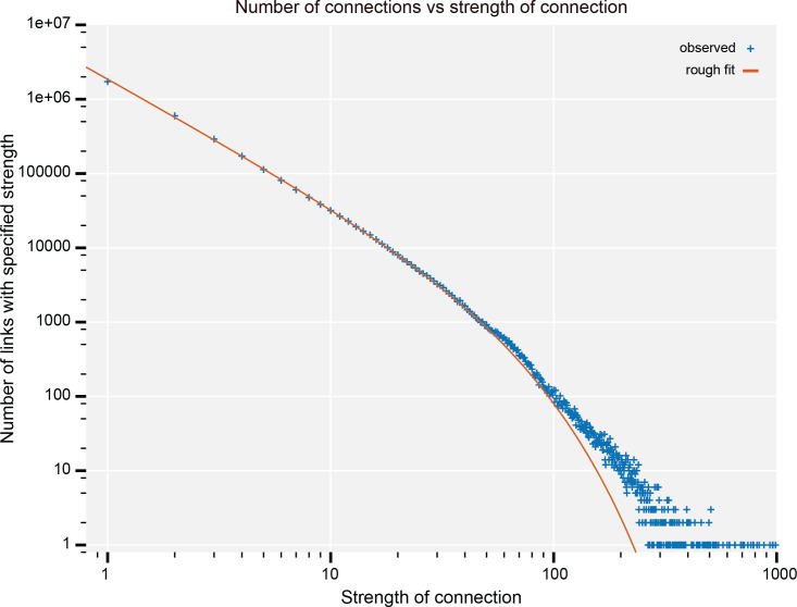
The neural circuits responsible for animal behavior remain largely unknown. We summarize new methods and present the circuitry of a large fraction of the brain of the fruit fly Drosophila melanogaster. Improved methods include new procedures to prepare, image, align, segment, find synapses in, and proofread such large data sets. We define cell types, refine computational compartments, and provide an exhaustive atlas of cell examples and types, many of them novel. We provide detailed circuits consisting of neurons and their chemical synapses for most of the central brain. We make the data public and simplify access, reducing the effort needed to answer circuit questions, and provide procedures linking the neurons defined by our analysis with genetic reagents. Biologically, we examine distributions of connection strengths, neural motifs on different scales, electrical consequences of compartmentalization, and evidence that maximizing packing density is an important criterion in the evolution of the fly's brain.

Keywords: D. melanogaster; brain regions; cell types; computational biology; connectome; connectome reconstuction methods; graph properties; neuroscience; synapse detecton; systems biology.

Plain language summary

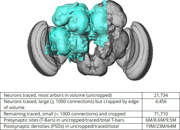
Animal brains of all sizes, from the smallest to the largest, work in broadly similar ways. Studying the brain of any one animal in depth can thus reveal the general principles behind the workings of all brains. The fruit fly Drosophila is a popular choice for such research. With about 100,000 neurons – compared to some 86 billion in humans – the fly brain is small enough to study at the level of individual cells. But it nevertheless supports a range of complex behaviors, including navigation, courtship and learning. Thanks to decades of research, scientists now have a good understanding of which parts of the fruit fly brain support particular behaviors. But exactly how they do this is often unclear. This is because previous studies showing the connections between cells only covered small areas of the brain. This is like trying to understand a novel when all you can see is a few isolated paragraphs. To solve this problem, Scheffer, Xu, Januszewski, Lu, Takemura, Hayworth, Huang, Shinomiya et al. prepared the first complete map of the entire central region of the fruit fly brain. The central brain consists of approximately 25,000 neurons and around 20 million connections. To prepare the map – or connectome – the brain was cut into very thin 8nm slices and photographed with an electron microscope. A three-dimensional map of the neurons and connections in the brain was then reconstructed from these images using machine learning algorithms. Finally, Scheffer et al. used the new connectome to obtain further insights into the circuits that support specific fruit fly behaviors. The central brain connectome is freely available online for anyone to access. When used in combination with existing methods, the map will make it easier to understand how the fly brain works, and how and why it can fail to work correctly. Many of these findings will likely apply to larger brains, including our own. In the long run, studying the fly connectome may therefore lead to a better understanding of the human brain and its disorders. Performing a similar analysis on the brain of a small mammal, by scaling up the methods here, will be a likely next step along this path.


Conflict of interest statement

LS, CX, ZL, ST, KH, GH, KS, SB, JC, PH, WK, LU, TZ, DA, JB, TD, DK, TK, KK, NN, DO, HO, ET, MI, AB, JG, TW, RS, PS, EN, CK, CA, DB, SB, JB, BC, NC, MC, MD, OD, BE, KF, SF, NF, AF, GH, EJ, SK, NK, JK, SL, AL, CM, EM, SM, CM, MN, OO, NO, CO, NP, CP, TP, EP, EP, NR, CR, MR, JR, SR, MS, AS, AS, AS, CS, KS, NS, MS, AS, JS, ST, IT, DT, ET, TT, JW, TY, JH, FL, RP, PR, VJ, MC, GJ, KI, SS, RG, IM, GR, HH, SP No competing interests declared, MJ, JM, TB, LL, PL, LL, VJ is an employee of Google.

Figures

Figure 1.
Figure 1.. The hemibrain and some basic statistics.
The highlighted area shows the portion of the central brain that was imaged and reconstructed, superimposed on a grayscale representation of the entire Drosophila brain. For the table, a neuron is traced if all its main branches within the volume are reconstructed. A neuron is considered uncropped if most arbors (though perhaps not the soma) are contained in the volume. Others are considered cropped. Note: (1) our definition of cropped is somewhat subjective; (2) the usefulness of a cropped neuron depends on the application; and (3) some small fragments are known to be distinct neurons. For simplicity, we will often state that the hemibrain contains ≈25K neurons.
Figure 2.
Figure 2.. The 13 slabs of the hemibrain, each flattened and co-aligned.
A vertical section at the level of the fan-shaped body is shown. Colors are arbitrary and added to the monochrome data to show brain regions, as defined below. Scale bar 50 μm.
Figure 3.
Figure 3.. Examples of results of CycleGAN processing.
(a) Original EM data from tab 34 at a resolution of 16 nm / resolution, (b) EM data after CycleGAN processing, (c–d) FFN segmentation results with the 16 nm model applied to original and processed data, respectively. Scale bar in (a) represents 1 μm.
Figure 4.
Figure 4.. Well-preserved membranes, darkly stained synapses, and smooth round neurite profiles are characteristics of the hemibrain sample.
Panel (A) shows polyadic synapses, with a red arrow indicating the presynaptic T-bar, and white triangles pointing to the PSDs. We identified in total 64 million PSDs and 9.5 million T-bars in the hemibrain volume (Figure 1). Thus the average number of PSDs per T-bar in our sample is 6.7. Mitochondria (‘M’), synaptic vesicles (‘SV’), and the scale bar (0.5 μm) are shown. Panel (B) shows a horizontal cross section through a point cloud of all detected synapses. This EM point cloud defines many of the compartments in the fly’s brain, much like an optical image obtained using antibody nc82 (an antibody against Bruchpilot, a component protein of T-bars) to stain synapses. This point cloud is used to generate the transformation from our sample to the standard Drosophila brain.
Figure 5.
Figure 5.. Precision and recall for synapse prediction, panel (A) for T-bars, and panel (B) for synapses as a whole including the identification of PSDs.
T-bar identification is better than PSD identification since this organelle is both more distinct and typically occurs in larger neurites. Each dot is one brain region. The size of the dot is proportional to the volume of the region. Humans proofreaders typically achieve 0.9 precision/recall on T-bars and 0.8 precision/recall on PSDs, indicated in purple. Data available in Figure 5—source datas 1–2.
Figure 6.
Figure 6.. Division of the sample into brain regions.
(A) A vertical section of the hemibrain dataset with synapse point clouds (white), predicted glial tissue (green), and predicted fiber bundles (magenta). (B) Grayscale image overlaid with segmented neuropils at the same level as (A). (C) A frontal view of the reconstructed neuropils. Scale bar: (A, B) 50 μm.
Figure 7.
Figure 7.. Reconstructed brain regions and substructures.
(A, B) Dorsal views of the olfactory projection neurons (PNs) and the innervated neuropils, AL, CA, and LH. Uniglomerular PNs projecting through the mALT are shown in (A), and multiglomerular PNs are shown in (B). (C, D) Columnar visual projection neurons. Each subtype of cells is color coded. LC cells are shown in (C), and LPC, LLPC, and LPLC cells are shown in (D). (E, F) The nine layers of the fan-shaped body (FB), along with the asymmetrical bodies (AB) and the noduli (NO), displayed as an anterior-ventral view (E), and a lateral view (F). In (E), three FB tangential cells (FB1D (blue), FB3A (green), FB8H (purple)) are shown as markers of the corresponding layers (FBl1, FBl3, and FBl8, respectively). (G) Zones in the ellipsoid body (EB) defined by the innervation patterns of different types of ring neurons. In this horizontal section of the EB, the left side shows the original grayscale data, and the seven ring neuron zones (see Table 1) are color-coded. The right side displays the seven segmented zones based on the innervation pattern, in a slightly different section. Scale bar: 20 μm.
Figure 8.
Figure 8.. Quality checks of the brain compartments.
(A) Areas of the boundaries (in square microns) between adjacent neuropils, indicated on a log scale. (B) The number of excess crossings normalized by the area of neuropil boundary. Larger dots indicate a more uncertain boundary. Data available in Figure 8—source data 1.
Figure 9.
Figure 9.. An example of two neurons with very similar shapes but differing connectivities.
PEN1 is on the left, PEN2 on the right.
Figure 10.
Figure 10.. Workflow for defining cell types.
Figure 11.
Figure 11.. The number of cell types in each major brain region.
The total number of cell types shown in this graph is larger than the total number of cell types shown in Table 3, because types that arborize in multiple regions are counted in each region in which they occur. Data available in Figure 11—source data 1.
Figure 12.
Figure 12.. Histogram showing the number of cell types with a given number of constituent cells.
Data available in Figure 12—source data 1.
Figure 13.
Figure 13.. Overview of the operation of CBLAST.
Figure 14.
Figure 14.. Cells of nine types plotted according to their connectivities.
Coordinates are in arbitrary units after dimensionality reduction using UMAP (McInnes et al., 2018). The results largely agree with those from morphological clustering but in some cases show separation even between closely related types.
Figure 15.
Figure 15.. Connection precision of upstream and downstream partners for ≈1000 cell types.
Data available in Figure 15—source data 1.
Figure 16.
Figure 16.. Difference between synapse counts in connections of the Ellipsoid Body, with increased completeness in proofreading.
Roughly 40,000 connection strengths are shown. Almost all points fall above the line Y = X, showing that almost all connections increased in synapse count, with very few decreasing. In particular, no path decreased by more than five synapses. Only two new strong (count >10) paths were found that were not present in the original. As proofreading proceeds, this error becomes less and less common since neuron fragments (orphans) are added in order of decreasing size (see text). Data available in Figure 16—source data 1.
Figure 17.
Figure 17.. Overview of data representations of our reconstruction.
Circles are stored data representations, rectangles are application programs, ellipses represent users, and arrows indicate the direction of data flow labeled with transformation and/or format. Filled areas represent existing technologies and techniques; open areas were developed for the express purpose of EM reconstruction of large circuits.
Figure 18.
Figure 18.. Schema for the neo4j graph model of the hemibrain.
Each neuron contains 0 or more SynapseSets, each of which contains one or more synapses. All the synapses in a SynapseSet connect the same two neurons. If the details of the synapses are not needed, the neuron-to-neuron weight can be obtained as a property on the ‘ConnectsTo’ relation, as can the distribution of this weight across different brain regions (the roiInfo).
Figure 19.
Figure 19.. Comparison of the size and orientation of brain images.
Sagittal section images at the plane of the mushroom body pedunculus are shown. Parallel lines indicate the direction of serial sectioning. Purple dotted lines indicate the axes of the pedunculus to show the sample orientation. Numbers indicate the angles of the pedunculus axes relative to the horizontal axis. Scale bar: 50 μm for all images. CA: calyx of the mushroom body. Panel (a) Hemibrain EM image stack. Grayscale indicates the density of the points of the presynaptic T-bars (point clouds). (b) Confocal light microscopy image stack provided by the Insect Brain Name Working Group (Ito et al., 2014), of a female brain mounted in 80% glycerol after antibody labeling. Presynaptic sites are labeled by GFP fused with the synaptic vesicle-associated protein neuronal synaptobrevin (nSyb), driven by the pan-neuronal expression driver line elav-GAL4 C155. (c) JRC2018 Unisex brain template (Bogovic et al., 2020), which is an average of 36 female and 26 male brains mounted in DPX plastic after dehydration with ethanol and clearization with xylene. Presynaptic sites are labeled with the SNAP chemical tag knock-in construct inserted into the genetic locus of the active zone protein bruchpilot (brp). The relative sizes of the brains, measured as the height along the lines that are perpendicular to the pedunculus axes, are 100:83:70 for (a), (b), and (c). These differences in size and orientation must be taken into account when comparing the sections and reconstructed neurons of the hemibrain EM and registered light microscopy images.
Figure 20.
Figure 20.. Plots of the percentage of pairs connected (of all possible) versus the number of interneurons required.
(a) It shows the data from the whole hemibrain, for up to eight interneurons. (b) It is a much wider view of the same data, shown on a log scale so the curve from a human designed system is visible. Data available in Figure 20—source datas 1–6.
Figure 21.
Figure 21.. The number of connections with a given strength.
Up to a strength of 100, this is well described by a power law (exponent −1.67) with exponential cutoff (at N = 42). Data available in Figure 21—source data 1.
Figure 22.
Figure 22.. Large motifs searched for.
Squares represent abundant types with at least 20 instances. Circles represent sparse types with at most two instances. Panel (a) shows a clique, where all possible connections are present. (b) It shows bidirectional connections between a sparse type and all instances of an abundant type. (c) It shows unidirectional connections from all of an abundant type to a sparse type. Panel (d) illustrates a cell type that does not form a clique overall, but does within each of two compartments.
Figure 23.
Figure 23.. One to many motifs found in the optic circuits.
Cell types consisting of a single cell, or a left-right pair, are shown at the top of the diagram. Corresponding cell type, each with many instances, are shown at the bottom of the diagram, with the number of cells per type shown inside. The arrows show the average count of synaptic connections per one cell of the bottom group. (a) An example of the most common case is shown. Here one cell, PLP008, has bidirectional connections to all 82 cells of type LC13. (b) It shows a single cell with exhaustive connections to several types. (c) It shows an alternative motif where several cells form these one-to-many connections.
Figure 24.
Figure 24.. Neural connection patterns.
(a) An EPG neuron, with arbors in three compartments. (b) Two neurons that connect in more than one compartment, in this case the calyx and the lateral horn. They are each pre- and postsynaptic to each other in both compartments.
Figure 25.
Figure 25.. Delay versus amplitude plots for a neuron.
(a) The linear response to inputs in the gall (GA) for an EPG neuron, which also has arbors in the ellipsoid body (EB) and the protocerebral bridge (PB). Each point in the modeled plot shows the time each response reached its peak amplitude (the delay), and the amplitude at that time, for an input injected at one of the PSDs in the gall. (b) Delays and amplitudes for gall to PB response, for all combinations of three values of cytoplasmic resistance RA and three values of membrane resistance RM. Data available in Figure 25—source datas 1–4.
Figure 26.
Figure 26.. Rent’s rule for the hemibrain.
The yellow region encompasses the theoretical bounds for computation. Four varieties of human-designed systems are shown. Those designed for visibility into computation achieve the upper bound, while those designed for minimum communication approach the lower bounds (Microprocessors ST7LU55, LPC1102, and STM32). Human designed systems where efficient packing is the main criterion occupy the shaded area (in 2D and 3D). The characteristics of the primary compartments completely contained in the reconstructed volume are shown with alphanumeric labels. The hemibrain compartments fall very nearly in the same range as human designed systems designed for efficient packing. Data available in Figure 26—source data 1.
Appendix 1—figure 1.
Appendix 1—figure 1.. Precision-recall plot of T-bar prediction.
The purple intercept indicates estimated manual agreement rate of 0.9. Data available in Appendix 1—figure 1—source data 1.
Appendix 1—figure 2.
Appendix 1—figure 2.. Precision-recall plot of end-to-end synapse prediction.
The purple intercept indicates estimated manual agreement rate of 0.8. Data available in Appendix 1—figure 2—source data 1.
Appendix 1—figure 3.
Appendix 1—figure 3.. Comparison of synful+ connection strength versus cascade connection strength (truncated at a connection strength of 500 for clarity, omitting 40 edges from each prediction set).
Data available in Appendix 1—figure 3—source data 1.

Comment in

  • Mapping the mind of a fly.
    Pipkin J. Pipkin J. Elife. 2020 Oct 8;9:e62451. doi: 10.7554/eLife.62451. Elife. 2020. PMID: 33030427 Free PMC article.

References

    1. Ache JM, Polsky J, Alghailani S, Parekh R, Breads P, Peek MY, Bock DD, von Reyn CR, Card GM. Neural basis for looming size and velocity encoding in the Drosophila giant fiber escape pathway. Current Biology. 2019;29:1073–1081. doi: 10.1016/j.cub.2019.01.079. - DOI - PubMed
    1. Altschul SF, Gish W, Miller W, Myers EW, Lipman DJ. Basic local alignment search tool. Journal of Molecular Biology. 1990;215:403–410. doi: 10.1016/S0022-2836(05)80360-2. - DOI - PubMed
    1. Ascoli GA, Donohue DE, Halavi M. NeuroMorpho.Org: a central resource for neuronal morphologies. Journal of Neuroscience. 2007;27:9247–9251. doi: 10.1523/JNEUROSCI.2055-07.2007. - DOI - PMC - PubMed
    1. Aso Y, Hattori D, Yu Y, Johnston RM, Iyer NA, Ngo TT, Dionne H, Abbott LF, Axel R, Tanimoto H, Rubin GM. The neuronal architecture of the mushroom body provides a logic for associative learning. eLife. 2014;3:e04577. doi: 10.7554/eLife.04577. - DOI - PMC - PubMed
    1. Auer TO, Benton R. Sexual circuitry in Drosophila. Current Opinion in Neurobiology. 2016;38:18–26. doi: 10.1016/j.conb.2016.01.004. - DOI - PubMed

Publication types

LinkOut - more resources