Satellite isoprene retrievals constrain emissions and atmospheric oxidation

Abstract

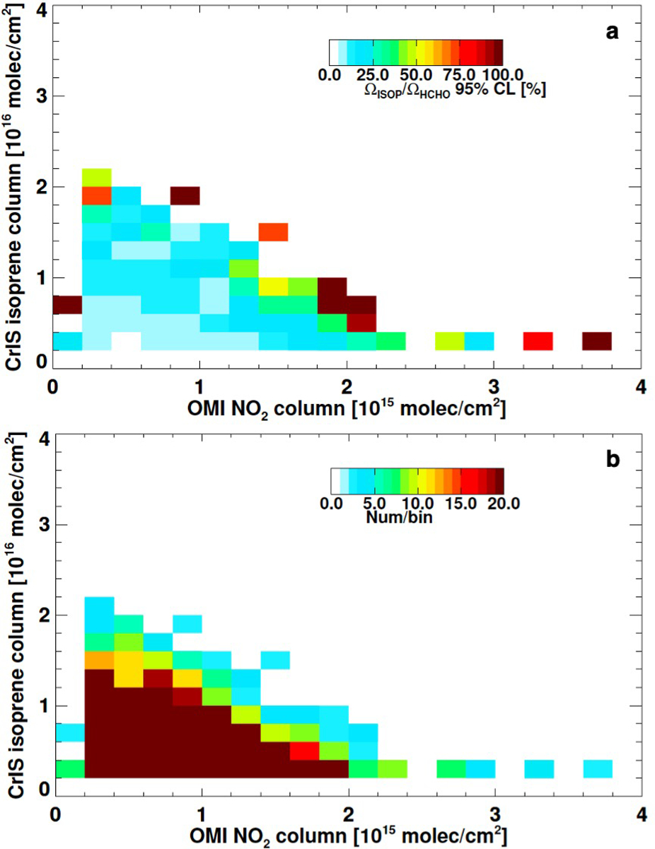
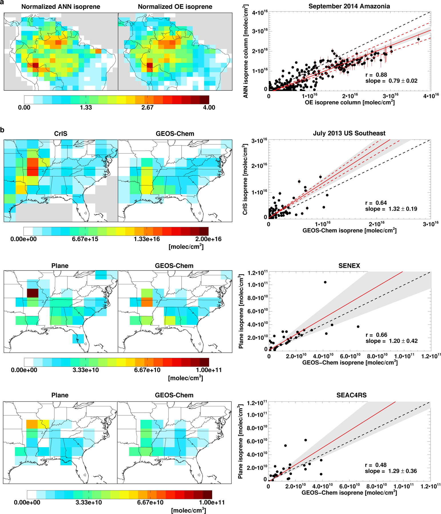
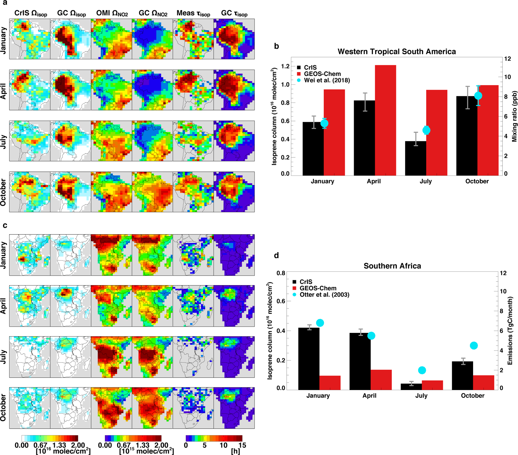
Isoprene is the dominant non-methane organic compound emitted to the atmosphere^1-3. It drives ozone and aerosol production, modulates atmospheric oxidation and interacts with the global nitrogen cycle^4-8. Isoprene emissions are highly uncertain^1,9, as is the nonlinear chemistry coupling isoprene and the hydroxyl radical, OH-its primary sink^10-13. Here we present global isoprene measurements taken from space using the Cross-track Infrared Sounder. Together with observations of formaldehyde, an isoprene oxidation product, these measurements provide constraints on isoprene emissions and atmospheric oxidation. We find that the isoprene-formaldehyde relationships measured from space are broadly consistent with the current understanding of isoprene-OH chemistry, with no indication of missing OH recycling at low nitrogen oxide concentrations. We analyse these datasets over four global isoprene hotspots in relation to model predictions, and present a quantification of isoprene emissions based directly on satellite measurements of isoprene itself. A major discrepancy emerges over Amazonia, where current underestimates of natural nitrogen oxide emissions bias modelled OH and hence isoprene. Over southern Africa, we find that a prominent isoprene hotspot is missing from bottom-up predictions. A multi-year analysis sheds light on interannual isoprene variability, and suggests the influence of the El Niño/Southern Oscillation.

Extended Data Fig. 1 |. Simulated spectral signals near 900 cm⁻¹ for the CrIS sensor.

a, Brightness temperature (T_b) difference for simulated spectra with and without isoprene (black), nitric acid (red), ammonia (blue), and CFC-12 (yellow), and a 10% perturbation in water vapor (green). Red and blue arrows indicate the ν₂₈ on-peak and off-peak spectral points used to calculate ΔT_b. Simulations were performed with LBLRTM^, for an isoprene profile with 5 ppb in the boundary layer (P > 800 hPa) that decays exponentially aloft, and AFGL US standard atmosphere profiles of temperature, water vapor, and nitric acid. b, Relationship between ΔT_b and isoprene column density, shaded by thermal contrast, for the full synthetic dataset used in this work. c, Global distribution of surface-atmosphere thermal contrast at the time of the CrIS overpass. Maps are derived from time-interpolated GMAO temperatures for January, April, July, and October.

Extended Data Fig. 2 |. CrIS isoprene measurements over Amazonia as derived using ANN- and OE-based approaches.

Data are shown for September 2014 and displayed as absolute columns.

Extended Data Fig. 3 |. Global distribution of isoprene columns, emissions, and lifetime as predicted by GEOS-Chem.

Predicted columns (left column), emissions (middle column), and lifetime (z < 500 m; right column) are shown at 1330 LT for January, April, July, and October 2013.

Extended Data Fig. 4 |. Statistical uncertainty in the global distribution of monthly mean isoprene:HCHO ratios as a function of isoprene and NO_x regime.

a, Relative 95% confidence interval in the mean ratio for each isoprene and tropospheric NO₂ bin. b, Number of observations in each bin.

Extended Data Fig. 5 |. Global distribution of isoprene column densities derived from CrIS.

Plotted are the mean (left column) and relative standard deviation (right column) across the 10 ANNs for January, April, July, and October 2013.

Extended Data Fig. 6 |

Boundaries of the four regions examined in the seasonal bar plots shown in Figs. 5 and 6.

Extended Data Fig. 7 |. Measured and simulated HCHO columns.

Plotted are the HCHO columns measured by OMI (left column) and simulated by GEOS-Chem (right column) at ~1330 LT for January, April, July, and October 2013.

Extended Data Fig. 8 |. CrIS cloud screening and ANN performance.

a, Function used for cloud screening CrIS L1B data prior to ΔT_b calculation. The black line shows the modeled clear-sky difference between the 900 cm⁻¹ brightness temperature and surface skin temperature, as a function of water vapor column density (calculated using LBLRTM^,). The solid red line is the linear approximation used here, and the dashed red line represents a less stringent threshold used to test the sensitivity of the results to our cloud screening approach. Panels b and c show the sensitivity of the CrIS brightness temperature differences (b) and isoprene columns (c) to cloud screening. Data shown represent the median relative differences between the base-case results (derived using the solid red line panel a) and those derived using the less stringent cloud screening threshold (dashed red line in panel a). Scatterplots show the predicted versus true isoprene columns for (d) the six-predictor ANN and (e) an ANN in which ΔT_b is withheld as a predictor variable. Red dots show the mean of the 10 ANN predictions, and blue error bars show the standard deviation across the predictions. f, The relative uncertainty (based on the difference between the mean ANN predicted value and the true value) for the six-predictor ANN, binned as a function of thermal contrast and isoprene column density.

Fig. 1 |. Global distribution of brightness temperature differences (ΔT_b) and isoprene columns.

Left column: monthly-mean ΔT_b observations from CrIS. Middle column: isoprene column densities derived from the CrIS observations. Right column: isoprene column densities simulated by GEOS-Chem. Data are plotted for January, April, July, and October 2013 at ~1330 LT (1200–1500 LT mean, with daily cloud screening applied). Ocean scenes are excluded from the isoprene maps as they are not part of the ANN training dataset (see Methods).

Fig. 2. |. Comparison of the CrIS artificial neural network (ANN) isoprene columns with other datasets.

a, Comparison of ANN- and optimal estimation (OE)-derived isoprene estimates. Both are derived from cloud-screened CrIS radiances for September 2014; ANN results employ GEOS-Chem HNO₃ as CrIS HNO₃ data were unavailable for this timeframe. The maps display columns normalized to their domain means, with the scatterplot comparing the absolute columns (absolute columns are mapped in Extended Data Fig. 2). b, Evaluation of CrIS ANN isoprene measurements using aircraft observations and GEOS-Chem model output. Top row: monthly-mean July 2013 isoprene columns as measured by CrIS (~1330 LT) and simulated by GEOS-Chem (1200–1500 LT mean). Bottom two rows: ambient isoprene concentrations as measured during the SENEX (June-July 2013; middle row) and SEAC⁴RS (August-September 2013; bottom row) aircraft campaigns and simulated by GEOS-Chem along the flight tracks. Data are plotted as campaign-average density-weighted boundary layer number densities (P > 800 hPa). In both a and b, error bars indicate the standard deviation across the 10 ANN-based columns (see Methods), red dashed lines indicate the range in slopes across ANNs, and black dashed lines indicate the 1:1 relation. Stated slope uncertainties and gray shaded regions represent the bootstrapped standard error of regression.

Fig. 3 |. Dependence of atmospheric isoprene columns on emissions and lifetime.

a, The global ensemble of monthly-mean ~1330 LT (1200–1500 LT mean) GEOS-Chem isoprene columns predicted for 2013 versus the corresponding isoprene emissions. b, The predicted isoprene:HCHO column ratio shown as a function of isoprene lifetime, 1/[OH], and [OH] (all for z < 500 m). Both plots are shaded by the modeled tropospheric NO₂ column.

Fig. 4 |. Global distribution of the isoprene:HCHO ratio (a proxy for 1/OH; Fig. 3) as a function of isoprene and NO_x.

a, the observed relationship based on CrIS and OMI. b, the simulated relationship from GEOS-Chem. In both cases the plotted ratios represent monthly mean values at 1330 LT (1200–1500 LT mean) and are binned by isoprene and tropospheric NO₂ column amounts. Data shown reflect scenes with elevated surface temperature (> 293K at satellite overpass) and where the isoprene and HCHO measurements are above detection limit (2 × 10¹⁵ molec cm⁻²).

Fig. 5 |. Seasonality of space-based isoprene over Amazonia and southern Africa.

Left panels (a, c) map the CrIS and GEOS-Chem isoprene columns, OMI and GEOS-Chem tropospheric NO₂ columns, and space-based and GEOS-Chem isoprene lifetimes (τ_isop, calculated from the isoprene:HCHO ratios via the Fig. S3 transfer functions) for January, April, July, and October 2013. The CrIS isoprene and space-based isoprene lifetimes are shown for snow-free, above detection limit scenes (Ω_isoprene, Ω_HCHO > 2 × 10¹⁵ molec cm⁻²). Right panels (b, d) show the regional mean CrIS (black; error bars indicate the range across ANN predictions) and GEOS-Chem (red) isoprene columns for western South America (b, regions defined in Extended Data Fig. 6) and southern Africa (d). Results for western tropical South America are compared to in-situ mixing ratios (cyan points and error bars show the 1200–1500 LT mean and standard deviation) measured from May 2014-January 2015 in the central Amazon Basin. In-situ data were unavailable for most of July, so the July CrIS values are compared to the in-situ mean for June 2014. Southern Africa results are compared to monthly isoprene emissions from a detailed regional inventory.

Fig. 6 |. Seasonality of space-based isoprene over the US Southeast and Australia.

Left panels (a, c) map the CrIS and GEOS-Chem isoprene columns, OMI and GEOS-Chem tropospheric NO₂ columns, and space-based and GEOS-Chem isoprene lifetimes (τ_isop, calculated from the isoprene:HCHO ratios via the Fig. S3 transfer functions) for January, April, July, and October 2013. The CrIS isoprene and space-based isoprene lifetimes are shown for snow-free, above detection limit scenes (Ω_isoprene, Ω_HCHO > 2 × 10¹⁵ molec cm⁻²). Right panels (b, d) show the regional mean CrIS (black; error bars indicate the range across ANN predictions) and GEOS-Chem (red) isoprene columns for the US Southeast (b, regions defined in Extended Data Fig. 6) and southeast Australia (d). US Southeast results are compared to 10-year mean (1999–2008) isoprene concentration measurements from Atlanta, Georgia (cyan; error bars indicate the 10-year standard deviation). Southeast Australian results are compared to measurements from the Sydney Particle Study. January and April CrIS values are compared to summer (1 February-7 March 2011) and autumn (14 April-14 May 2012) campaign means, respectively.

References

1. Guenther AB et al. The Model of Emissions of Gases and Aerosols from Nature version 2.1 (MEGAN2.1): an extended and updated framework for modeling biogenic emissions. Geosci. Model Dev 5, 1471–1492, doi:10.5194/gmd-5-1471-2012 (2012). - DOI
1. Saunois M et al. The global methane budget 2000–2012. Earth Syst. Sci. Data 8, 697–751, doi:10.5194/essd-8-697-2016 (2016). - DOI
1. Huang GL et al. Speciation of anthropogenic emissions of non-methane volatile organic compounds: a global gridded data set for 1970–2012. Atmos. Chem. Phys 17, 7683–7701, doi:10.5194/acp-17-7683-2017 (2017). - DOI
1. Trainer M et al. Models and observations of the impact of natural hydrocarbons on rural ozone. Nature 329, 705–707, doi:10.1038/329705a0 (1987). - DOI
1. Hewitt CN et al. Ground-level ozone influenced by circadian control of isoprene emissions. Nat. Geosci 4, 671–674, doi:10.1038/ngeo1271 (2011). - DOI
Publication types