PLANETARY CANDIDATES OBSERVED BY Kepler. VIII. A FULLY AUTOMATED CATALOG WITH MEASURED COMPLETENESS AND RELIABILITY BASED ON DATA RELEASE 25

Abstract

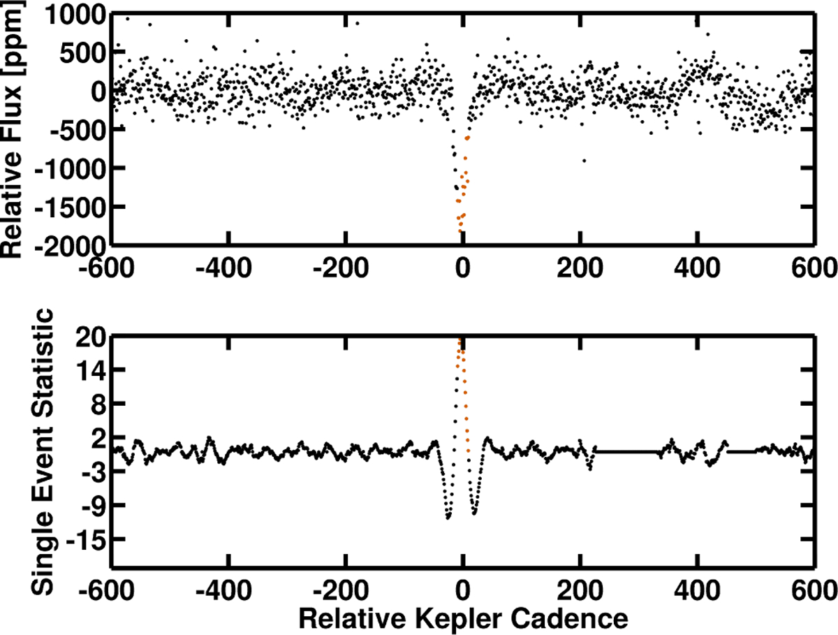
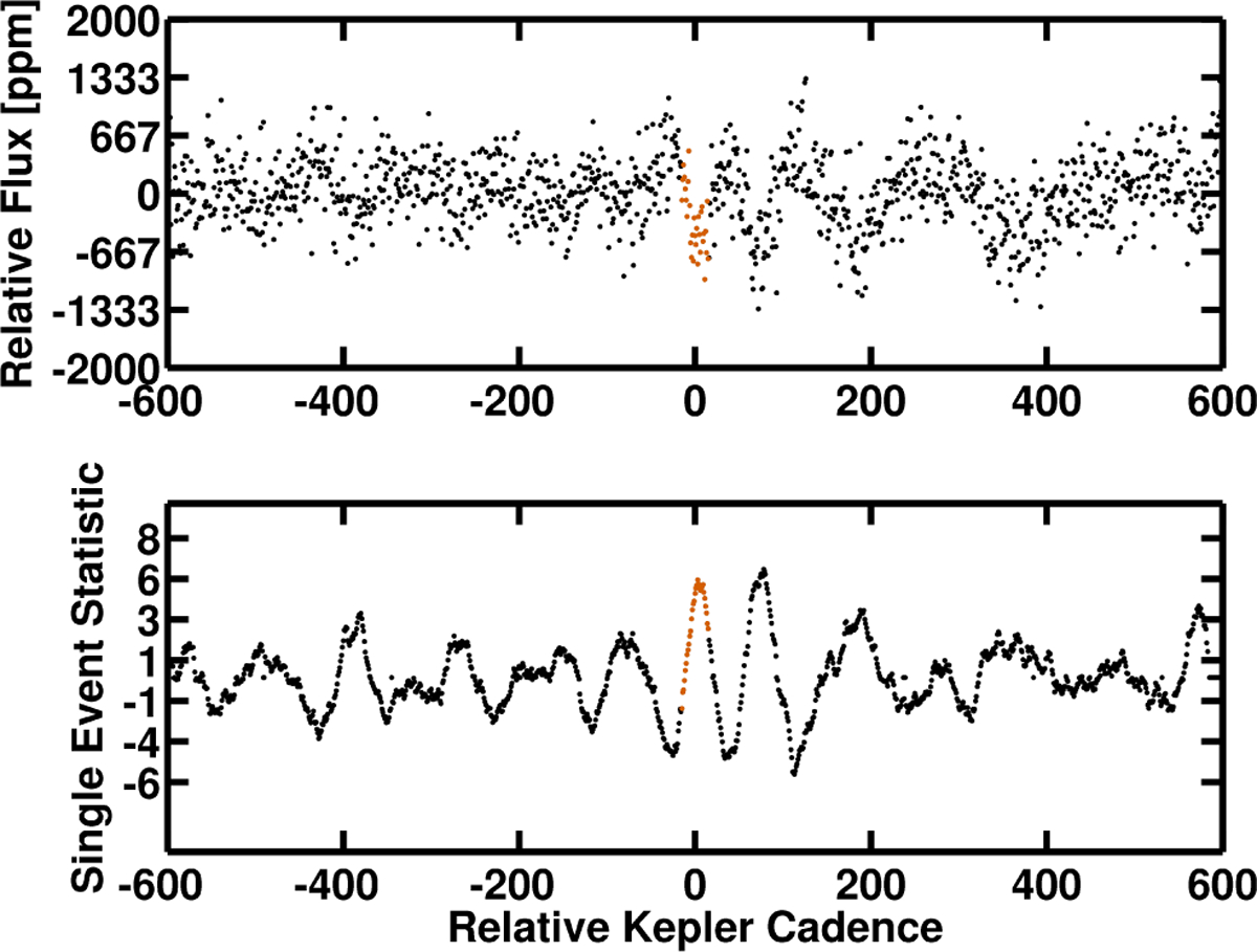
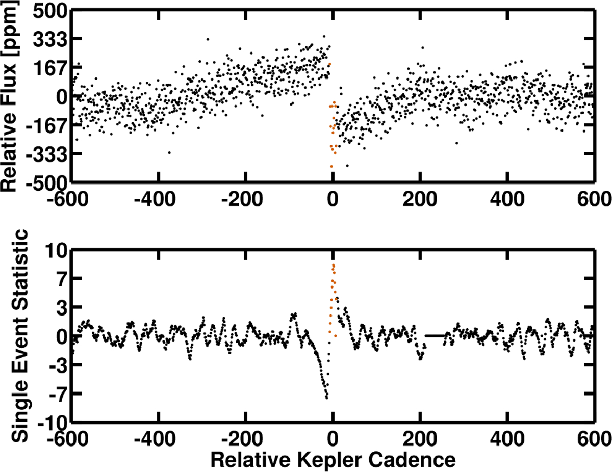
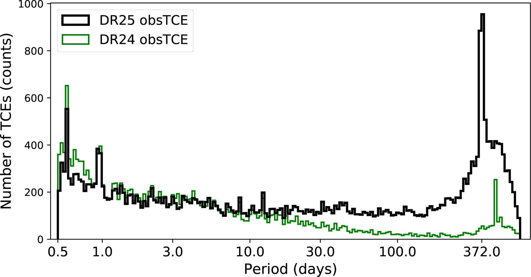
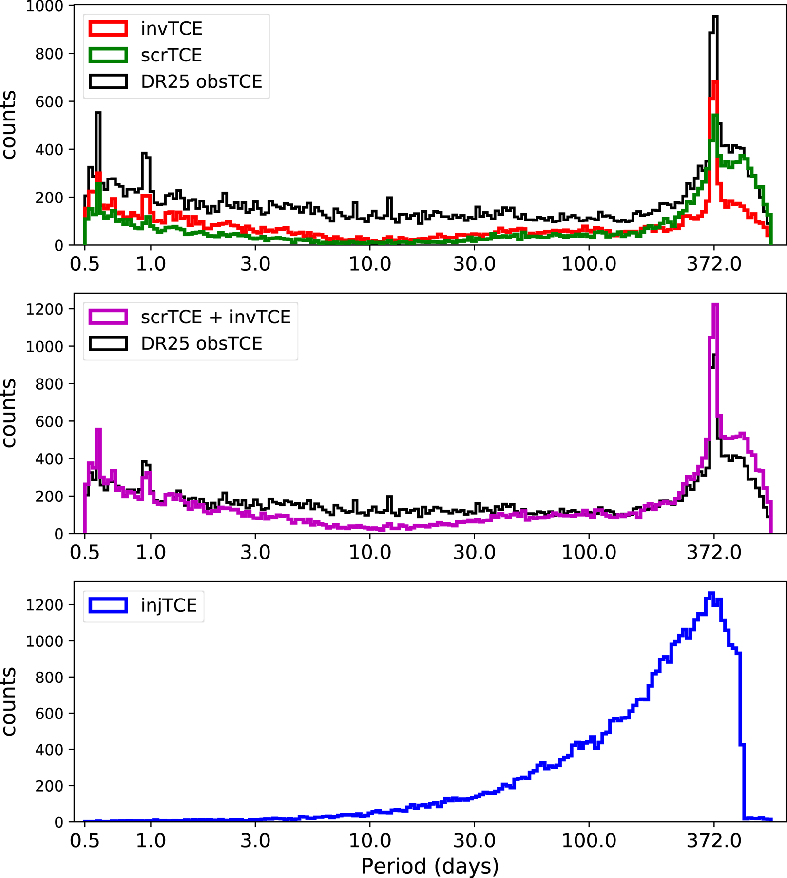
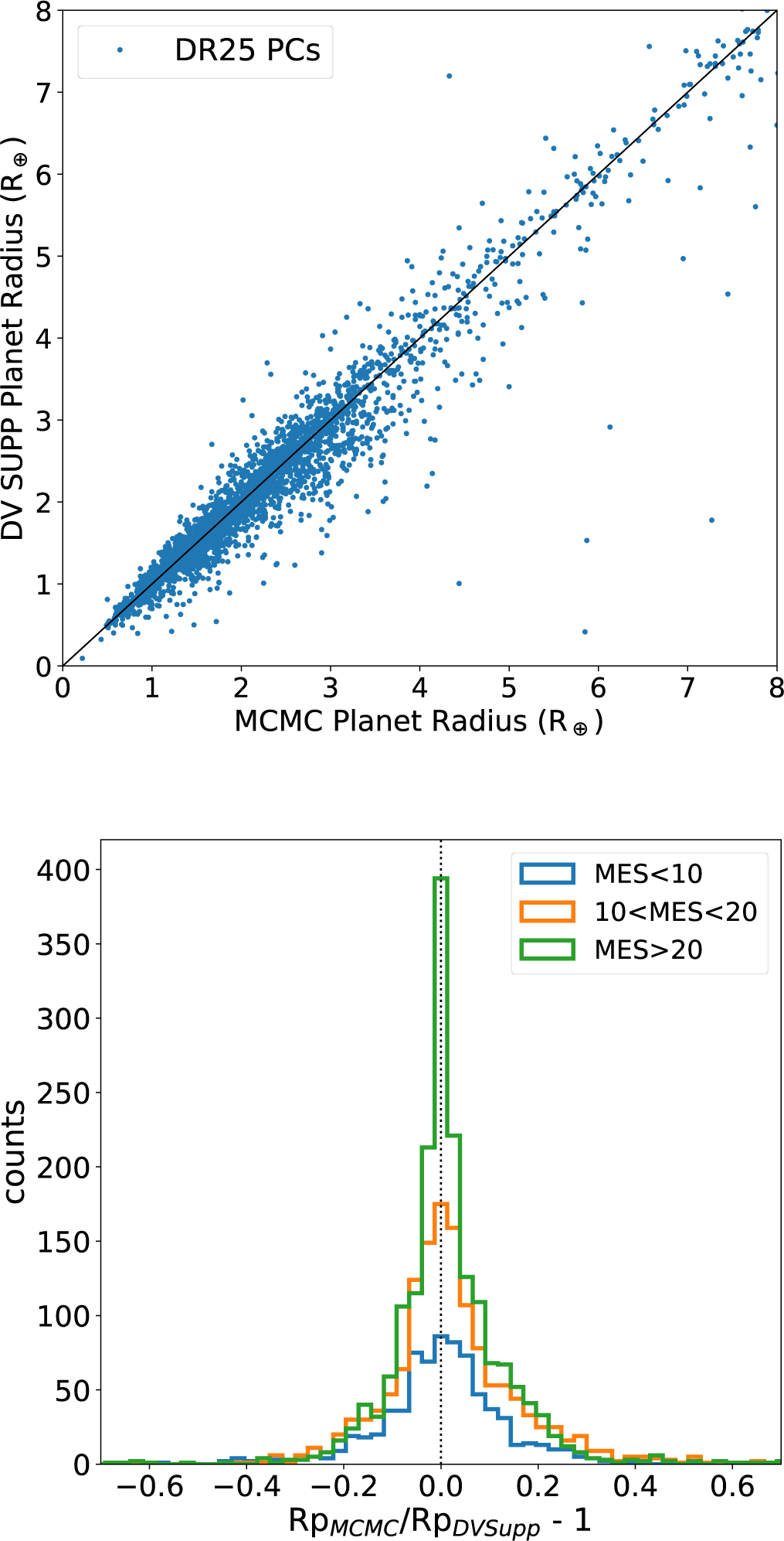
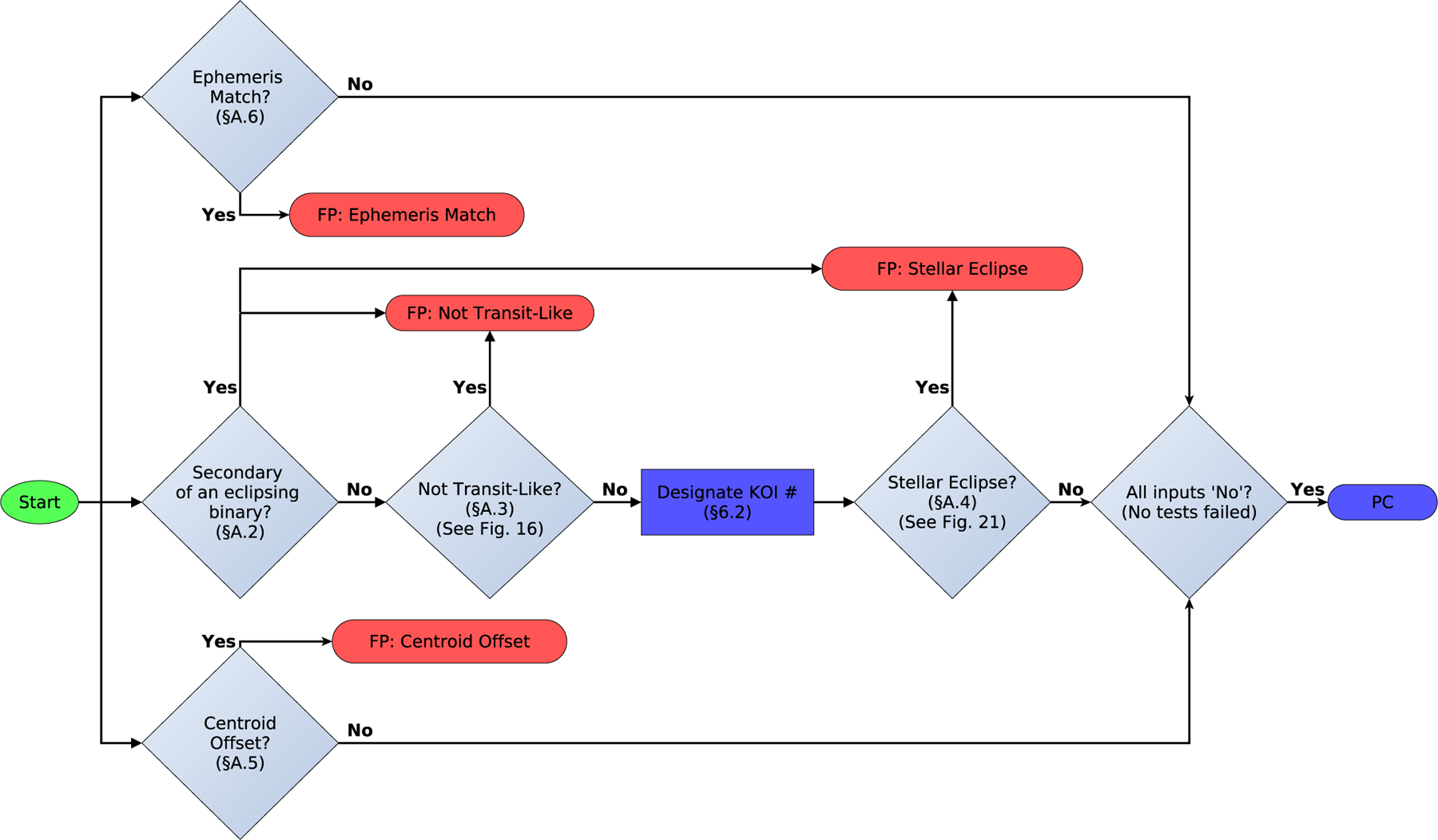
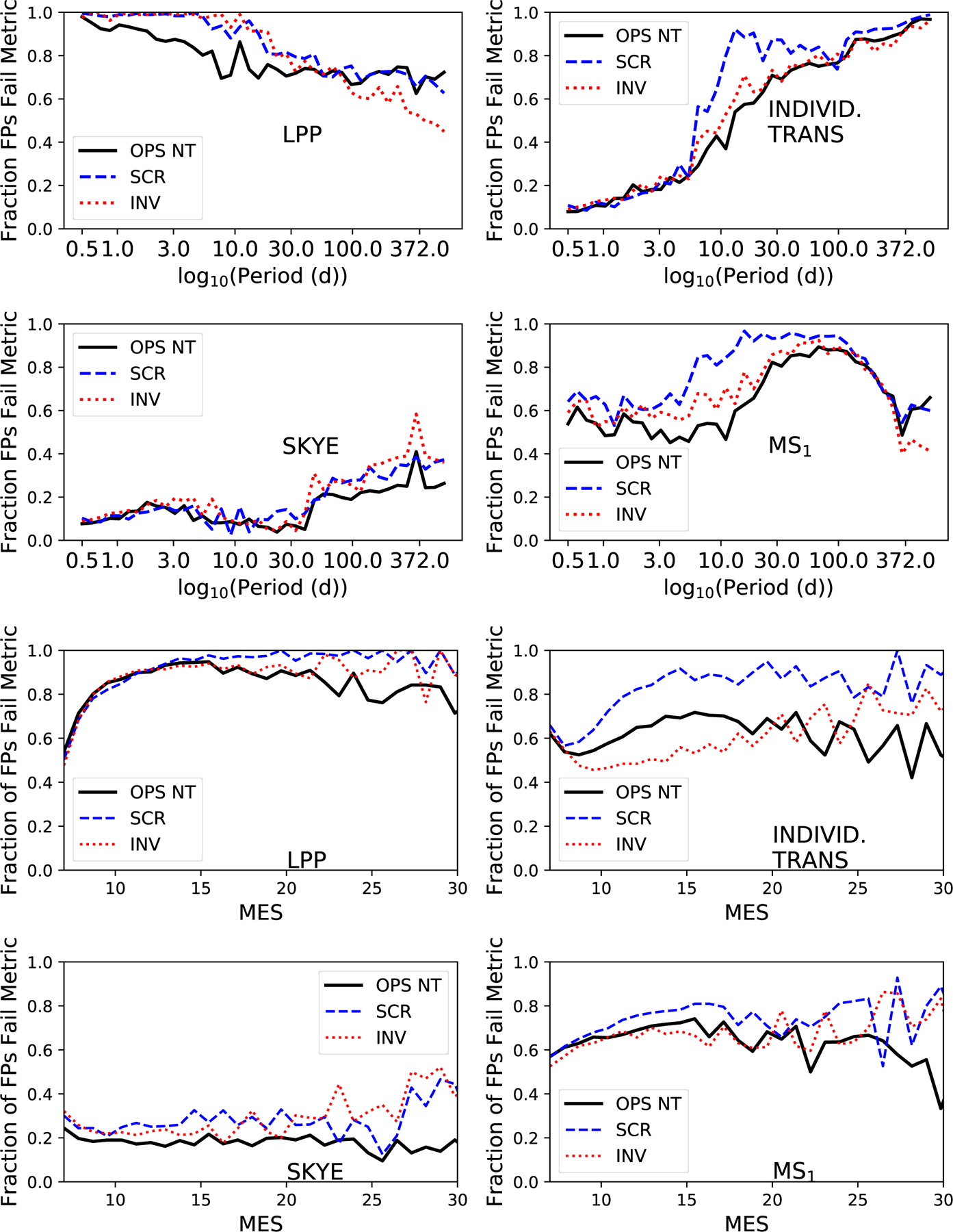
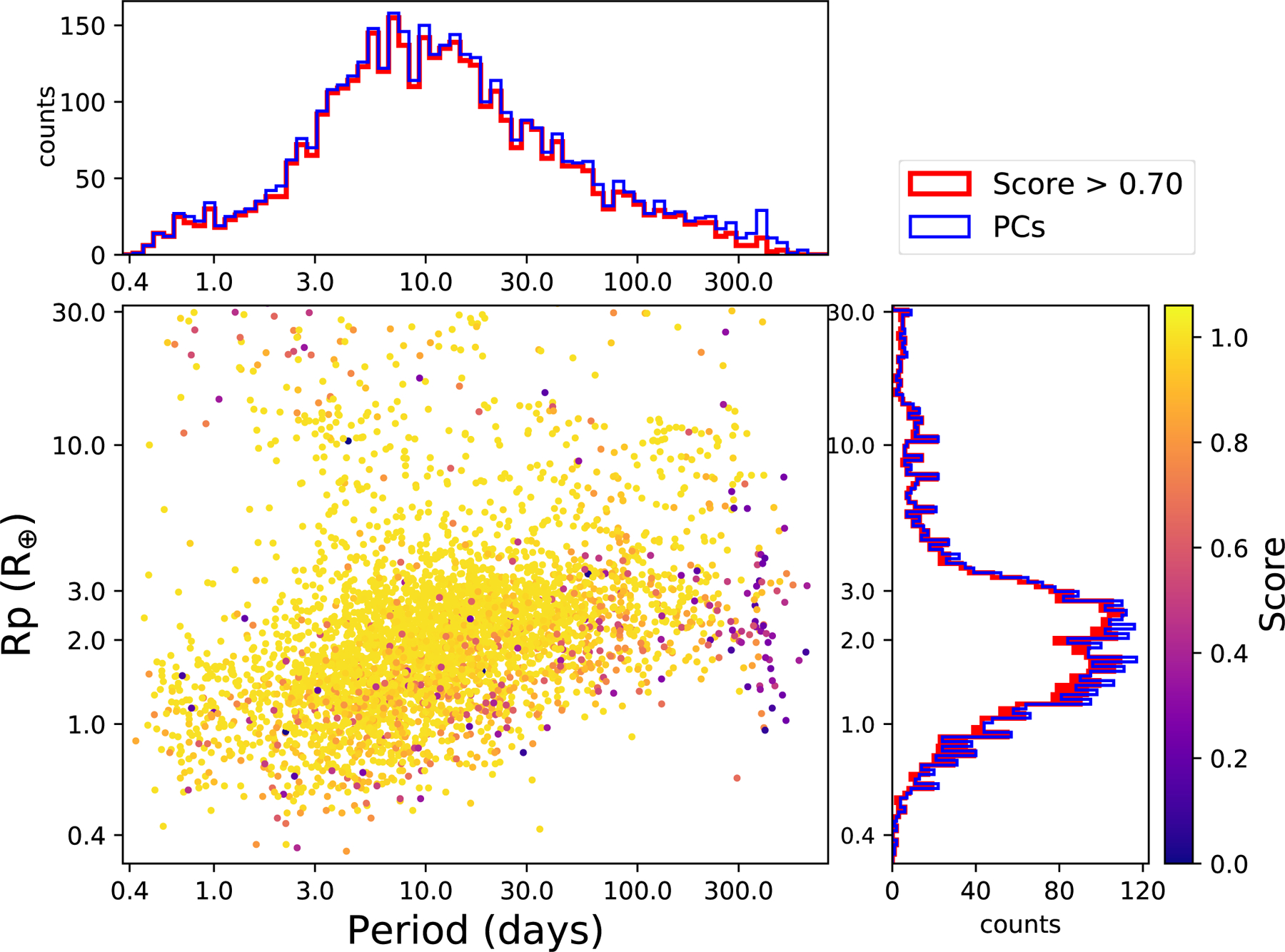
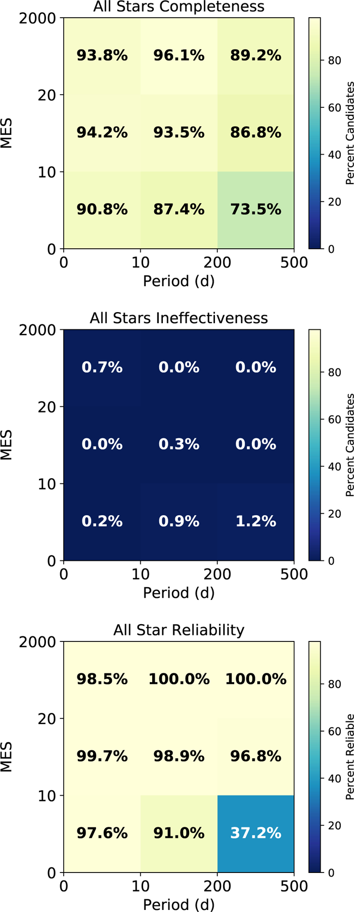
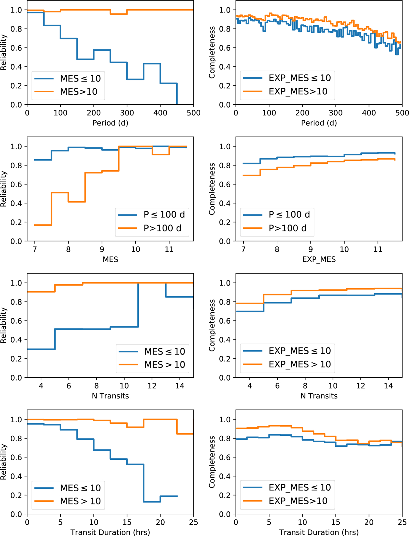
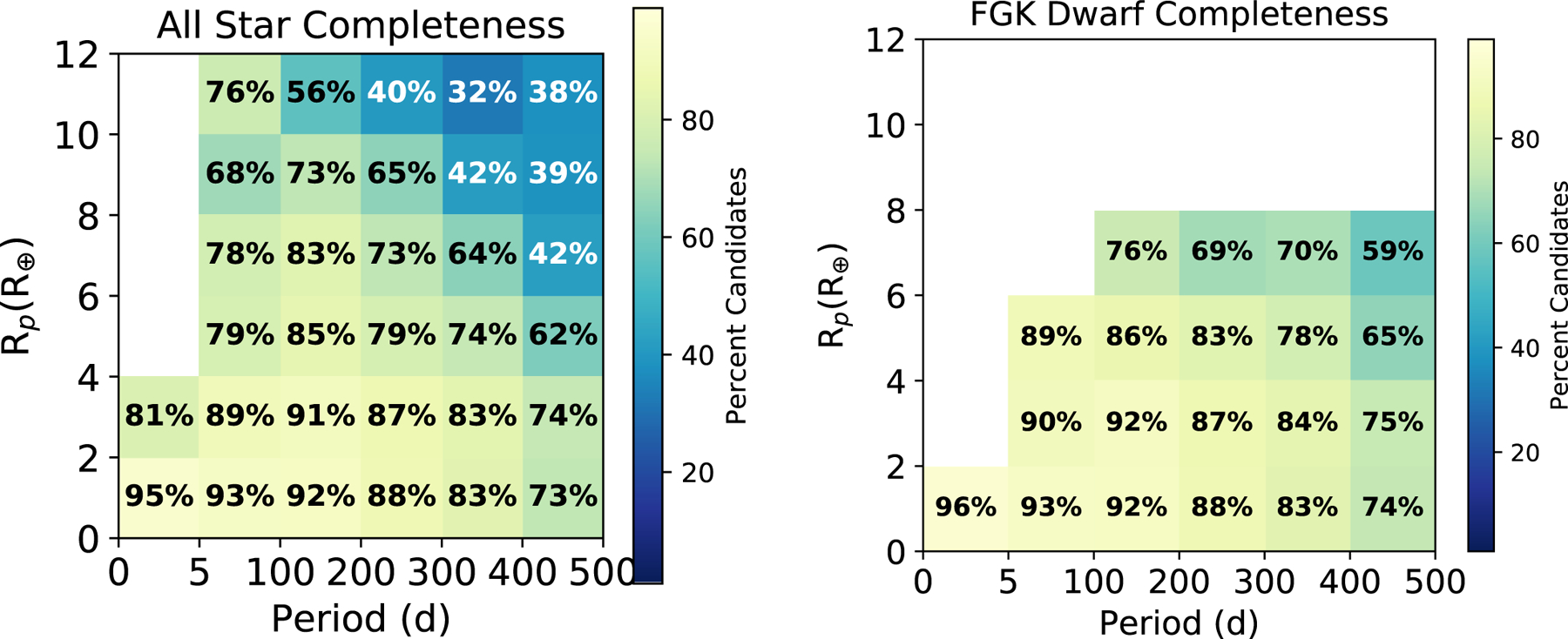
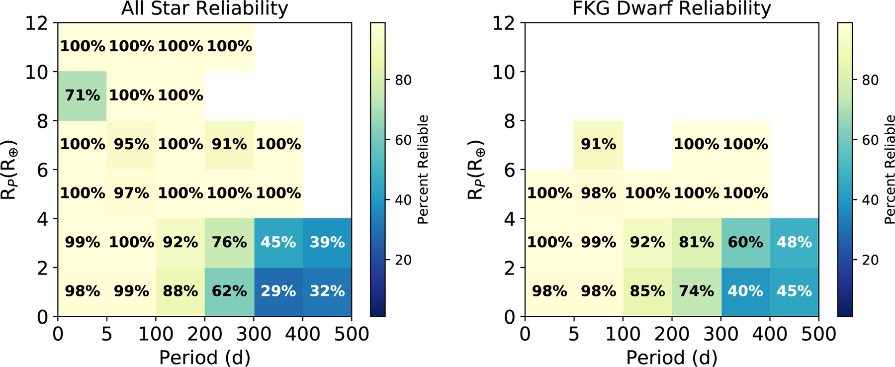
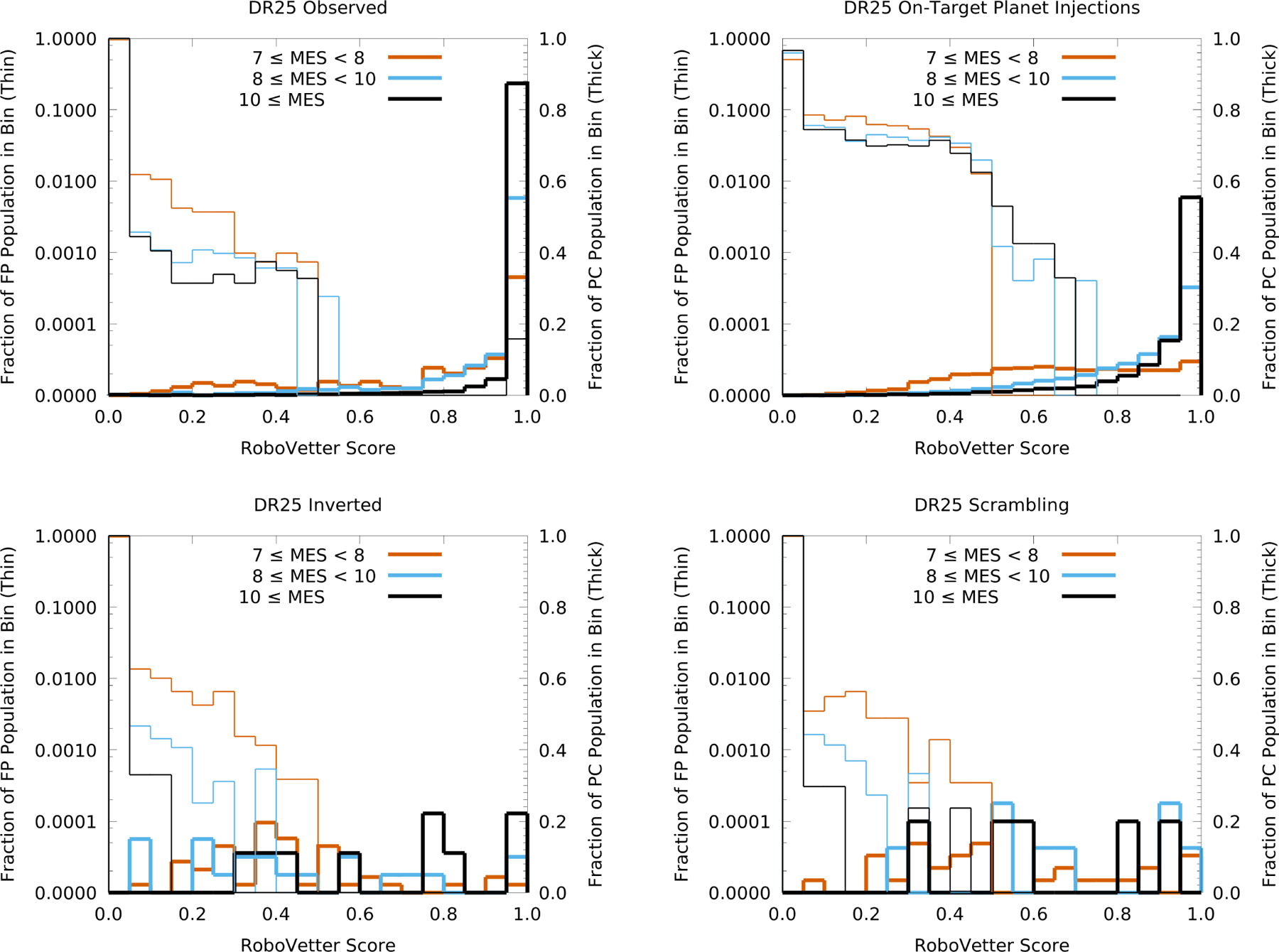
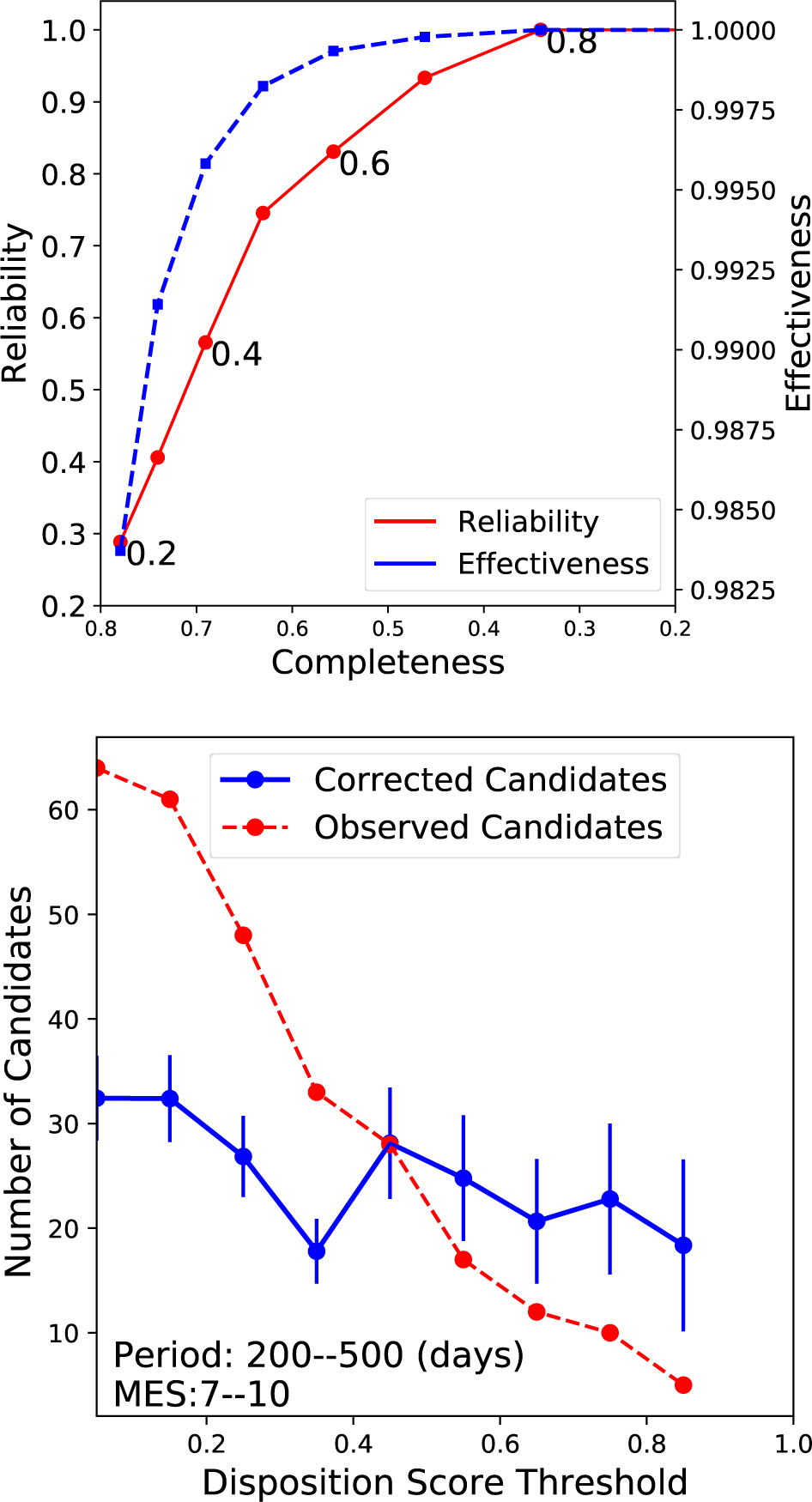
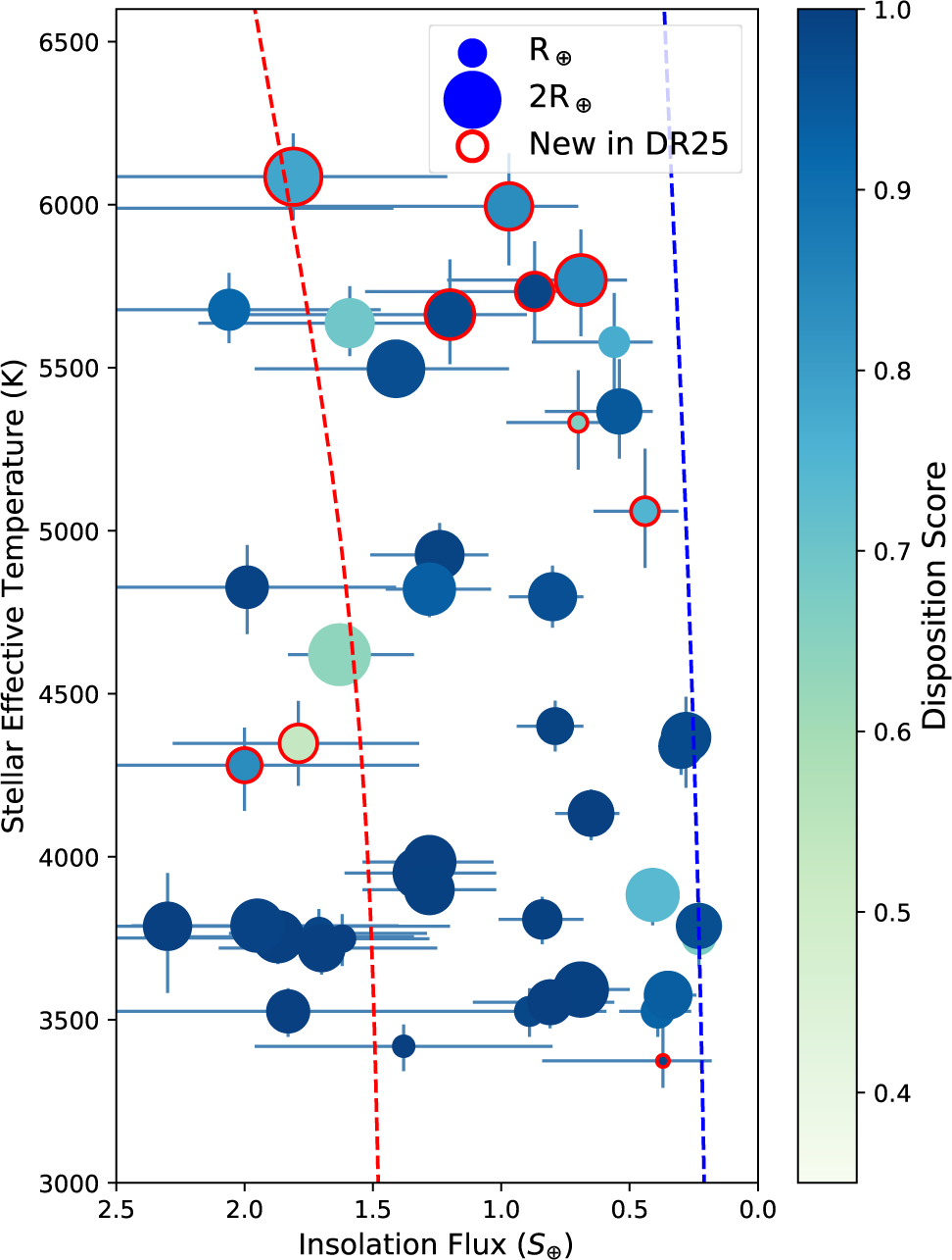
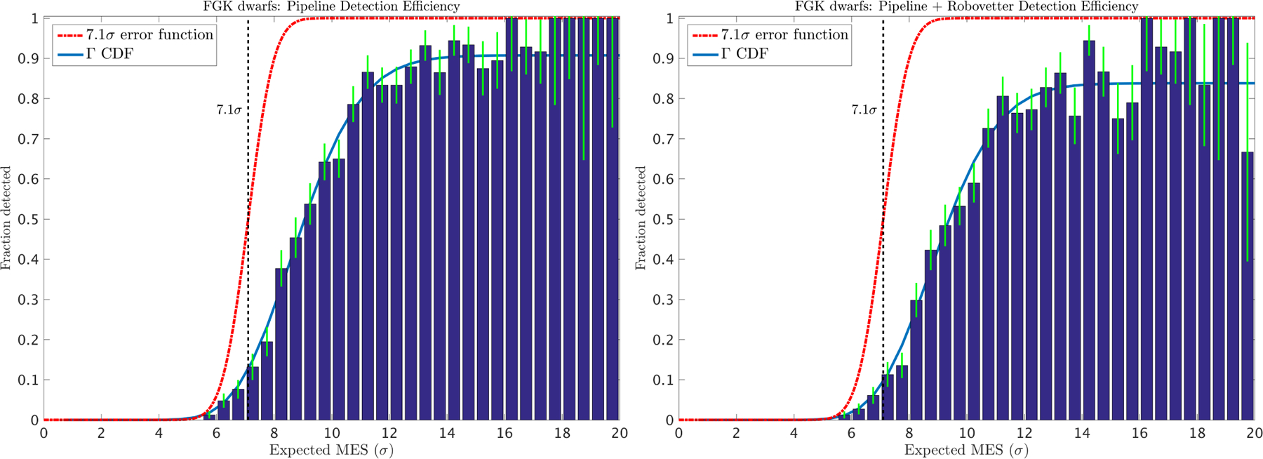
We present the Kepler Object of Interest (KOI) catalog of transiting exoplanets based on searching four years of Kepler time series photometry (Data Release 25, Q1-Q17). The catalog contains 8054 KOIs of which 4034 are planet candidates with periods between 0.25 and 632 days. Of these candidates, 219 are new in this catalog and include two new candidates in multi-planet systems (KOI-82.06 and KOI-2926.05), and ten new high-reliability, terrestrial-size, habitable zone candidates. This catalog was created using a tool called the Robovetter which automatically vets the DR25 Threshold Crossing Events (TCEs) found by the Kepler Pipeline (Twicken et al. 2016). Because of this automation, we were also able to vet simulated data sets and therefore measure how well the Robovetter separates those TCEs caused by noise from those caused by low signal-to-noise transits. Because of these measurements we fully expect that this catalog can be used to accurately calculate the frequency of planets out to Kepler's detection limit, which includes temperate, super-Earth size planets around GK dwarf stars in our Galaxy. This paper discusses the Robovetter and the metrics it uses to decide which TCEs are called planet candidates in the DR25 KOI catalog. We also discuss the simulated transits, simulated systematic noise, and simulated astrophysical false positives created in order to characterize the properties of the final catalog. For orbital periods less than 100 d the Robovetter completeness (the fraction of simulated transits that are determined to be planet candidates) across all observed stars is greater than 85%. For the same period range, the catalog reliability (the fraction of candidates that are not due to instrumental or stellar noise) is greater than 98%. However, for low signal-to-noise candidates found between 200 and 500 days, our measurements indicate that the Robovetter is 73.5% complete and 37.2% reliable across all searched stars (or 76.7% complete and 50.5% reliable when considering just the FGK dwarf stars). We describe how the measured completeness and reliability varies with period, signal-to-noise, number of transits, and stellar type. Also, we discuss a value called the disposition score which provides an easy way to select a more reliable, albeit less complete, sample of candidates. The entire KOI catalog, the transit fits using Markov chain Monte Carlo methods, and all of the simulated data used to characterize this catalog are available at the NASA Exoplanet Archive.

Keywords: catalogs; planetary systems; planets and satellites: detection; stars: statistics; surveys; techniques: photometric.

Figure 16.

The not transit-like flowchart of the Robovetter. Diamonds represent “yes” or “no” decisions that are made with quantitative metrics. If a TCE fails any test (via a “yes” response to any decision) then it is dispositioned as a not transit-like FP. If a TCE passes all tests (via a “no” response to all decisions), then it is given a KOI number and passed to the stellar eclipse module (see §A.4 and Figure 21). The section numbers on each decision diamond correspond to the sections in this paper where these tests are discussed.

Figure 17.

Upper panel: flux time series for a single transit event contributing to the TCE for KOI 3900.01 on target KIC 11911580 (black points). The cadences in transit (orange points) show a significant flux decrement relative to the baseline flux level. Lower panel: SES time series of the transit event show in the upper panel, representing the archetypal shape of a transit signal displaying a strong central peak with two low-amplitude, symmetric side troughs. There are no other events as strong as the transit nearby in time so this signal has an individual transit event Chases metric, Ch_i = 1.

Figure 18.

Upper panel: flux time series for a single transit event contributing to the TCE on target KIC 11449918 (black points). The cadences in transit (orange points) show a flux decrement, but there are numerous other flux decrements of similar depth and shape. The instrumental “rolling band” pattern noise contributes systematics to the flux time series of target KIC 11449918 causing numerous signal detections. Lower panel: SES time series of the transit event shown in the upper panel, representing the non-unique nature of the SES peak relative to surrounding data. The neighboring peak of comparable strength in the SES time series would result in Ch_i = .016 and the transit would be considered “bad” by Chases.

Figure 19.

Upper panel: flux time series for a single transit event contributing to the TCE on target KIC 12357074 (black points). The cadences in transit (orange points) show a flux decrement, but the sudden drop in flux followed by the gradual return to the baseline is archetypal of the SPSD instrumental signature. Lower panel: SES time series for the transit event shown in the upper panel, illustrating the strongly asymmetric SES peak having a comparable amplitude negative SES trough preceding the SES peak. The neighboring trough of comparable absolute strength to the transit’s peak would result in Ch_i = .005 and the transit would be considered “bad” by Chases.

Figure 20.

An example of how the Skye metric flags individual transit events. The plots show the number of individual transit events (from TCEs with periods greater than 45 days) that occur in one-day time bins throughout the mission duration. Two of the 84 skygroups were chosen to be shown as examples, with skygroup 55 plotted on top, and skygroup 58 plotted on bottom. Skygroup 58 (lower panel) has a strong clustering of transit events at times that correspond to the ~372 day orbital period of the spacecraft, as the stars belonging to skygroup 58 fall on CCD channels with strong rolling-band signal. In contrast, skygroup 55 is nearly uniform. Individual transits that occur in a one-day time bin with a number of transit events above the threshold (shown by the blue horizontal line; see Equation A12) are flagged as bad transits due to the Skye metric.

Figure 21.

Flowchart describing the stellar eclipse tests of the Robovetter. Diamonds represent “yes” or “no” decisions that are made with quantitative metrics. The multiple arrows originating from “Start” represent decisions that are made in parallel.

Figure 22.

A plot of injected versus recovered periods and epochs of injected on-target planets. The top plots shows the difference between the injected and recovered periods (top) and epochs (right) as a function of period. The bottom plots show the measured standard deviation of the differences in period (left) and epoch (right) in logarithmic space. The red line shows the best-fit power-law in each case.

Figure 23.

Distribution of ephemeris matches on the focal plane. Symbol size scales with magnitude, while color represents the catalog in which the contaminating source was found. Blue indicates that the true transit is from a variable star only known as a result of ground-based observations. Red circles are stars listed in the Kepler EBWG catalog (Kirk et al. 2016, http://keplerebs.villanova.edu/), green are KOIs, and black are TCEs. Black lines connect false positive matches with the most likely contaminating parent. In most cases parent and child are so close that the connecting line is invisible.

Figure 1.

Histogram of the period in days of the DR25 obsTCEs (black) using uniform bin space in the base ten logarithm of the period. The DR24 catalog obsTCEs (Seader et al. 2015) are shown in green for comparison. The number of long-period TCEs is much larger for DR25 and includes a large spike in the number of TCEs at the orbital period of the spacecraft (372 days). The long and short period spikes for both distributions are discussed in §2.1.

Figure 2.

Histogram of the period in days of the cleaned invTCEs (top, red), the cleaned scrTCEs (top, green), and injTCEs (bottom, blue) in uniform, base-ten logarithmic spacing. The middle plot shows the union of the invTCEs and the scrTCEs in magenta. The DR25 obsTCEs are shown for comparison on the top two figures in black. At shorter periods (< 30 days) in the top figure, the difference between the simulated false alarm sets and the observed data represents the number of transit-like KOIs; at longer periods we primarily expect false alarms. Notice that the invTCEs do a better job of reproducing the one-year spike, but the scrTCEs better reproduce the long-period hump. Because the injTCEs are dominated by long-period events (significantly more long-period events were injected), we are better able to measure the Robovetter completeness for long-period planets than short-period planets.

Figure 3.

Top: Comparison of the DR25 PCs fitted planet radii measured by the MCMC fits and the DV supplemental fits. The 1:1 line is drawn in black. Bottom: Histogram of the difference between the MCMC fits and the DV fits for the planet candidates in different MES bins. While individual objects have different fitted values, as a group the planet radii from the two fits agree.

Figure 4.

Overview flowchart of the Robovetter. Diamonds represent “yes” or “no” decisions that are made with quantitative metrics. A TCE is dispositioned as an FP if it fails any test (a “yes” decision) and is placed in one or more of the FP categories. (A TCE that is identified as being the secondary eclipse of a system is placed in both the Not Transit-Like and Stellar Eclipse categories.) If a TCE passes all tests (a “no” decision for all tests) it is dispositioned as a PC. The section numbers on each component correspond to the sections in this paper where these tests are discussed. More in-depth flowcharts are provided for the not transit-like and stellar eclipse modules in Figures 16 and 21.

Figure 5.

The top-left plot shows the LPP_DV values of all on-target injected planets on FGK dwarf targets as a function of period, and the top-right shows them as a function of MES. The middle-left plots shows the measured positive 1σ deviation (in the same units as LPP_DV) as a function of MES and period, and the middle-right plot shows the resulting best-fit model. The bottom plots show the same thing, but for the negative 1σ deviation (again in the same units as LPP_DV). These resulting model distributions are used when computing the Robovetter disposition score.

Figure 6.

The fraction of not-transit-like FPs failed by a particular Robovetter metric plotted against the logarithm of the period (top two rows) or linear MES (bottom two rows). The fraction is plotted for the obsTCE set in black, the scrTCE set in blue, and the invTCE set in red. The metric under consideration is listed on each plot. For each metric we include fails from either detrending (DV or ALT). Upper left: LPP metric failures. Upper Right: TCEs that fail after removing a single transit due to any of the individual transit metrics. Lower left: TCEs that fail after removing a single transit due to the Skye metric. Lower right: Model Shift 1 metric failures. Notice that there is a basic similarity between the trends seen in the three data sets, especially at long periods and low MES.

Figure 7.

DR25 PCs plotted as planet radius versus period with the color representing the disposition score. The period and planet radii distributions are plotted on the top and on the left, respectively, in blue. The red line shows the distributions of those PCs with a disposition score greater than 0.7. The excess of PCs at long-periods disappears when cutting the population on disposition score.

Figure 8.

A coarse binning of the completeness (C), ineffectiveness (1-E), and reliability (R) for different period and MES bins (shown from top to bottom, respectively). The effectiveness and reliability are based on the combined invTCE and scrTCE data sets. Notice that the Robovetter effectiveness at removing these false alarms is incredibly high, but for long periods and low MES the resulting reliability is lower because of the large number of false alarms and small number of true planets. For FGK dwarf stars only, the reliability is 50.3% and the completeness is 76.7% for planets in the longest period, lowest MES box.

Figure 9.

The reliability (left) and completeness (right) of the DR25 catalog plotted as a function of period, MES, number of transits, and transit duration. In each case the blue line is for those with MES ≤ 10 or periods ≤ 100 d. The orange line shows the completeness or reliability for the rest of the population (see the legend for each plot). EXP_MES is the expected MES (see Christiansen 2017 and §7.3.1).

Figure 10.

The Robovetter completeness binned by period and planet radius for all stars (left) and for only FGK dwarf stars (right). Bins with fewer than 10 injTCEs are not plotted.

Figure 11.

A 2D binning of the candidate catalog reliability for period and planet radius for all stars (left) and for the FGK dwarf stars (right). Bins with fewer than 3 candidates or fewer than 20 simulated false alarms (from invTCE and scrTCE) are not plotted.

Figure 12.

Plots of the score distribution of PCs (thick lines, right y-axis) and FPs (thin lines, left y-axis, logarithmic scaling) for the observed (top-left), on-target planet injections (top-right), inverted (bottom-left), and scrambled (bottom-right) TCEs.

Figure 13.

[Top] The reliability (red) and effectiveness (blue) of the DR25 catalog as a function of Completeness for MES ≤ 10 and periods between 200 and 500 d PCs that result when using different disposition score thresholds (shown as black numbers) to select the PCs. Higher disposition score thresholds result in higher reliability but lower completeness. Note, the completeness axis increases to the left. [Bottom] The number of PCs (in red) in the same period and MES space when making a cut on different disposition scores. The blue line corrects the number of candidates for the completeness and reliability. The error bars only reflect a Poisson error based on the number of observed planet candidates shown in red.

Figure 14.

DR25, eta-Earth sample of PCs plotted as stellar effective temperature against insolation flux using the values reported in the DR25 KOI catalog (which uses stellar properties from the DR25 stellar catalog (Mathur et al. 2017). The size of the exoplanet is indicated by the size of the circle. The color indicates the disposition score. Only those with disposition score greater than 0.5 are plotted. Only objects whose error bars indicate that they could be in the habitable zone and have a radius less than 1.8 R_⊕ are shown. Those with a red ring are new to the DR25 catalog.

Figure 15.

Left: The average detection efficiency of the Kepler Pipeline for a sample of FGK stars, as measured by the pixel-level transit injection experiment and described by Christiansen (2017). The solid blue line is a best-fit Γ cumulative distribution function (see Equation 1 of Christiansen et al. 2016); the red dashed line shows the hypothetical performance for a perfect detector in TPS. Right: The average detection efficiency of the Kepler Pipeline and the Robovetter, where the injections successfully recovered by the Pipeline are then subsequently evaluated as PCs by the Robovetter.

References

1. Aigrain S, Llama J, Ceillier T, et al. 2015, MNRAS, 450, 3211
1. Akeson RL, Chen X, Ciardi D, et al. 2013, PASP, 125, 989
1. Ambikasaran S, Foreman-Mackey D, Greengard L, Hogg DW, & O’Neil M 2014, ArXiv e-prints, arXiv:1403.6015 - PubMed
1. Barclay T, Rowe JF, Lissauer JJ, et al. 2013, Nature, 494, 452. - PubMed
1. Barge P, Baglin A, Auvergne M, et al. 2008, A&A, 482, L17