. 2020 Sep 10;10(1):14890.
doi: 10.1038/s41598-020-71692-6.

Understanding diaschisis models of attention dysfunction with rTMS

Affiliations

Understanding diaschisis models of attention dysfunction with rTMS

Javier O Garcia et al. Sci Rep. .

Abstract

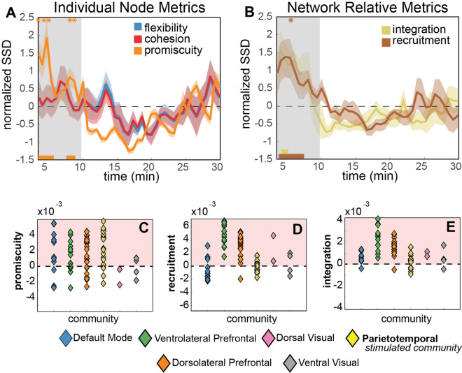
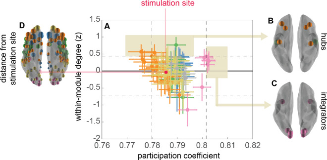
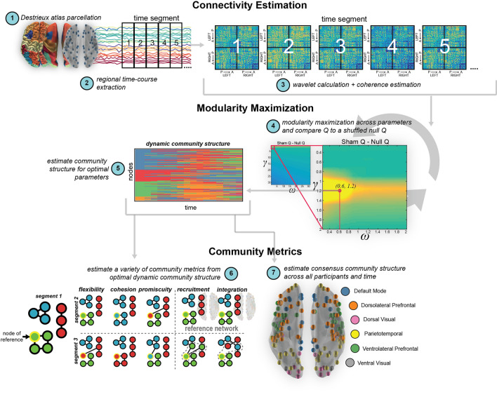
Visual attentive tracking requires a balance of excitation and inhibition across large-scale frontoparietal cortical networks. Using methods borrowed from network science, we characterize the induced changes in network dynamics following low frequency (1 Hz) repetitive transcranial magnetic stimulation (rTMS) as an inhibitory noninvasive brain stimulation protocol delivered over the intraparietal sulcus. When participants engaged in visual tracking, we observed a highly stable network configuration of six distinct communities, each with characteristic properties in node dynamics. Stimulation to parietal cortex had no significant impact on the dynamics of the parietal community, which already exhibited increased flexibility and promiscuity relative to the other communities. The impact of rTMS, however, was apparent distal from the stimulation site in lateral prefrontal cortex. rTMS temporarily induced stronger allegiance within and between nodal motifs (increased recruitment and integration) in dorsolateral and ventrolateral prefrontal cortex, which returned to baseline levels within 15 min. These findings illustrate the distributed nature by which inhibitory rTMS perturbs network communities and is preliminary evidence for downstream cortical interactions when using noninvasive brain stimulation for behavioral augmentations.


Conflict of interest statement

The authors declare no competing interests.

Figures

Figure 1
Figure 1
Community architecture during visual tracking, as assessed in the sham condition. Region centroids are represented as orbs plotted on a semi-transparent inflated brain. Colors indicate the consensus community structure, or the most common network architecture found across time and participants. Results indicate that on average this community structure is most common across time and participants with, on average, an 84.6% similarity in partitioning of this community structure to the others across participants and time.
Figure 2
Figure 2
Nodal community affiliation metrics in the rTMS and sham conditions. (AC) Average metric for each node across participants for each of the estimated individual nodal metrics, plotted with the corresponding color of the representative community as indicated by the legend. Circular gray region denotes metrics scores expected by chance (see Population distributions of node metrics in “Statistical significance” section for calculation specifics). Those scores exceeding 95% of the estimated null distribution are shown as larger tokens exceeding the null region. Semi-transparent inflated mesh brains inlayed in the upper left and lower right of each panel illustrate the spatial location of the nodes with metrics more extreme than expected by chance, with the size of the node scaled to the relative strength of the metric score. Images in the upper left of each panel show associated metric score as assessed in the sham condition and those in the bottom right are from the TMS condition.
Figure 3
Figure 3
rTMS-related nodal and motif dynamics. (A) Time-dependent changes in node metrics (flexibility, cohesion, promiscuity) following rTMS. Normalized SSD is the sum of squared differences (SSD) between sham and rTMS conditions, aggregated over all community nodes. Error bars indicate standard error of the between-subject means, computed from individual participant z-scored SSD timeseries. Metrics are estimated in approximately 40 s windows for concatenated 12 min scans. The shaded region isolates the first 10 min following stimulation during which the metrics most strongly deviate from the community structure as evaluated during Sham baseline. Bars along the bottom axis represent significant time points (uncorrected) from as single sample t-test, with color indicating metric (e.g. orange = promiscuity). Asterisks (*) at the top of the figure indicate significant time points following an FDR correction for multiple comparisons (i.e. time point comparisons). (B) Recruitment (stability vs flexibility) and integration (connectedness vs isolation) coefficients over time. (CE) Promiscuity, recruitment and integration computed during the first 10 min following rTMS (vs sham), shown for each node and organized by community.
Figure 4
Figure 4
Changes in promiscuity and allegiance metrics immediately following rTMS. Color maps correspond to the top 20% regional increases of these metrics within 10 min of the delivery of rTMS. Top row: dorsal view. Bottom row: ventral view. (A) Nodes with greatest increase in promiscuity included bilateral dorsal precentral cortex, orbitofrontal and middle temporal cortices. (B,C) Nodes with the highest integration (left) and recruitment coefficients (right) include anterior cingulate, bilateral orbitofrontal and fusiform, and precentral sulcus (recruitment only).
Figure 5
Figure 5
Characterizing the stimulation site. (A) Scatterplot of within-module degree and participation coefficients. Vertical dotted lines mark the central 90% of the participation coefficient across the brain (~ 133 nodes), and horizontal lines mark the central 90% of the within-module degree across all nodes all possible 148 regions. (B) Orbs plotted at the centroid of the regions that show the 95th percentile of the within-module degree, designating the most ‘hub-like’ nodes within the brain. (C) Orbs plotted at the centroid of the regions that show the 95th percentile of the participation coefficient, representing the ‘integrating’ nodes within the brain. (D) Orbs plotted at the centroid of all regions of the parcellated Destriuex atlas, where the size of node is scaled by the distance from the stimulation site or from the homologous region in the opposite hemisphere. The stimulation site (left intraparietal sulcus) is organized within the larger parietal, ventral temporal and orbitofrontal community (PT; shown in yellow).
Figure 6
Figure 6
Experimental task. Participants (A) were cued to attend to one of the four pinwheel wedges in each hemifield, (B) then tracked those wedges through 3 s of rotation at a speed individually calibrated for 85% accuracy (3 up, 1 down staircase procedure, conducted prior to stimulation). One pinwheel terminated in an upright position and (C) participants indicated which of the four wedges (up, down, left or right) corresponded to the cued wedge. (D) The mean changes in tracking accuracy following rTMS (as compared to sham baseline) for the contralateral and ipsilateral hemifields. The impact of rTMS on behavior was most apparent in the first experimental run of tracking, contralateral to the stimulation site (in the right visual field). Error bars indicate SE mean difference (TMS-Sham). (E) A bootstrap analysis in which run and hemifield labels were discarded to generate null distributions of expected change in performance (10,000 iterations) shows only 12.7% and 4.5% of contralateral and ipsilateral scores, respectively, have larger effect size than the impact of rTMS on contralateral tracking in the first experimental run (~ 12 min).
Figure 7
Figure 7
Dynamic community detection overview. Schematic of the approximate 7 steps completed for the dynamic community detection and metric estimation within this dataset. Briefly, (1) cortical regions of interest were parceled using the Destrieux atlas and (2) average regional time-courses were extracted from each of the 148 regions for each participant. (3) Timecourses were then passed through a continuous wavelet transformation and coherence was estimated between each pair of regions. (4) These connectivity matrices were then subjected to dynamic community detection across a set of parameters to determine the optimal “scale” in the dynamic community architecture. (5) A final community affiliation was calculated for the ‘optimal’ parameters, and these temporal labels were then used to (6) estimate community metrics (e.g., flexibility, cohesion, promiscuity, recruitment, and integration) and a representative community structure across participants (7).

Similar articles

Cited by

References

    1. Buschman TJ, Kastner S. From behavior to neural dynamics: an integrated theory of attention. Neuron. 2015;88:127–144. doi: 10.1016/j.neuron.2015.09.017. - DOI - PMC - PubMed
    1. Corbetta M, Shulman GL. Spatial neglect and attention networks. Annu. Rev. Neurosci. 2011;34:569–599. doi: 10.1146/annurev-neuro-061010-113731. - DOI - PMC - PubMed
    1. Husain M, Nachev P. Space and the parietal cortex. Trends Cogn. Sci. 2007;11:30–36. doi: 10.1016/j.tics.2006.10.011. - DOI - PMC - PubMed
    1. Stone SP, Halligan PW, Greenwood RJ. The incidence of neglect phenomena and related disorders in patients with an acute right or left hemisphere stroke. Age Ageing. 1993;22:46–52. doi: 10.1093/ageing/22.1.46. - DOI - PubMed
    1. Corbetta M, Kincade MJ, Lewis C, Snyder AZ, Sapir A. Neural basis and recovery of spatial attention deficits in spatial neglect. Nat. Neurosci. 2005;8:1603–1610. doi: 10.1038/nn1574. - DOI - PubMed

Publication types