. 2020 Sep 11;11(1):4568.
doi: 10.1038/s41467-020-18381-0.

Autoreservoir computing for multistep ahead prediction based on the spatiotemporal information transformation

Affiliations

Autoreservoir computing for multistep ahead prediction based on the spatiotemporal information transformation

Pei Chen et al. Nat Commun. .

Abstract

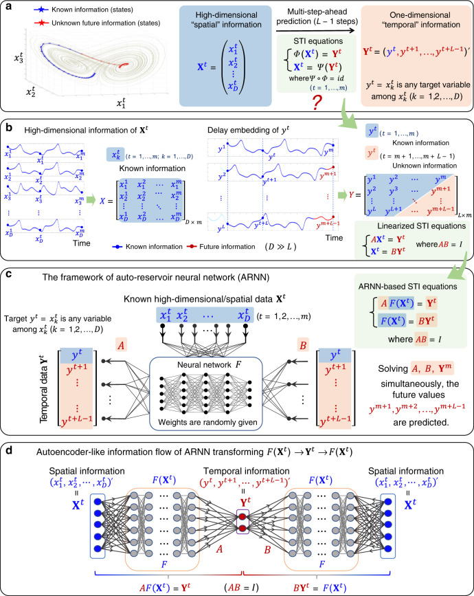
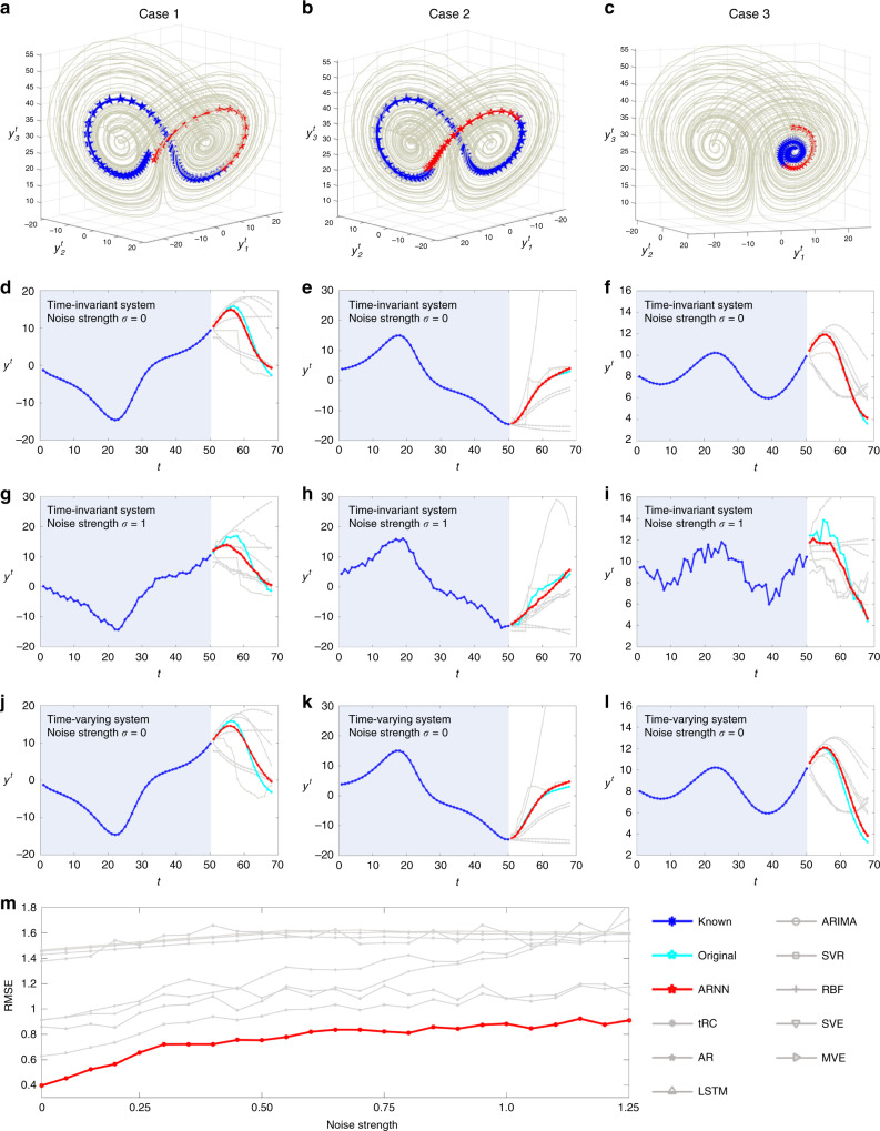
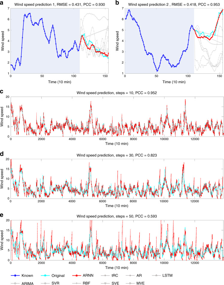
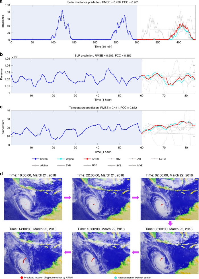
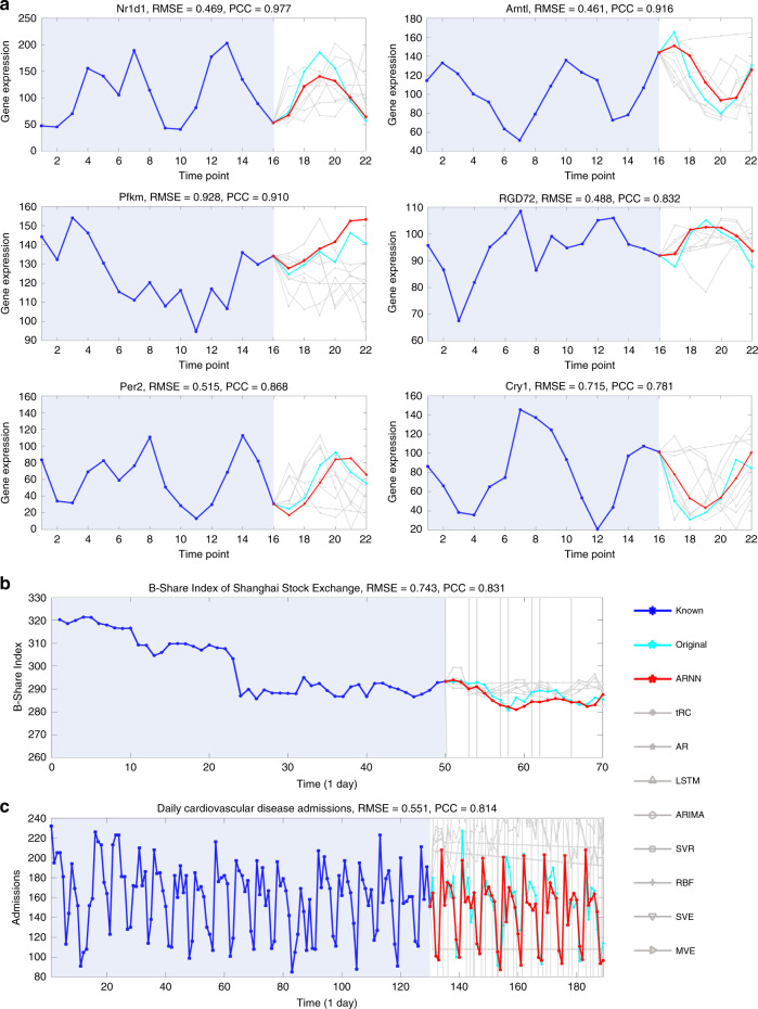
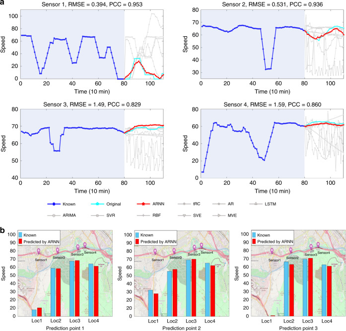
We develop an auto-reservoir computing framework, Auto-Reservoir Neural Network (ARNN), to efficiently and accurately make multi-step-ahead predictions based on a short-term high-dimensional time series. Different from traditional reservoir computing whose reservoir is an external dynamical system irrelevant to the target system, ARNN directly transforms the observed high-dimensional dynamics as its reservoir, which maps the high-dimensional/spatial data to the future temporal values of a target variable based on our spatiotemporal information (STI) transformation. Thus, the multi-step prediction of the target variable is achieved in an accurate and computationally efficient manner. ARNN is successfully applied to both representative models and real-world datasets, all of which show satisfactory performance in the multi-step-ahead prediction, even when the data are perturbed by noise and when the system is time-varying. Actually, such ARNN transformation equivalently expands the sample size and thus has great potential in practical applications in artificial intelligence and machine learning.


Conflict of interest statement

The authors declare no competing interests.

Figures

Fig. 1
Fig. 1. Schematic illustration of the auto-reservoir neural network.
a Given a short-term time series of a high-dimensional system, it is a challenging task to predict future states of any target variable. For a target variable y to be predicted, a delay-embedding strategy is applied, forming a delayed-coordinate vector Yt corresponding to the observed vector Xt via a function Φ. Such a relation constitutes the spatiotemporal information (STI) transformation with both primary and conjugate forms (STI equations). b The linearized STI equations also have primary and conjugate forms. Data can be represented in a matrix form where the future/unknown information {ym+1,ym+2,,ym+L1} is located in the lower-right triangle of matrix Y and the known information {y1, y2, …, ym} in the upper-left part of Y. c Auto-reservoir neural network (ARNN) is a model-free method to make the multistep-ahead prediction for a target y. In the ARNN framework, the reservoir component contains a random/fixed multilayer neural network F, for which there are time-dependent inputs Xt. A target vector Yt formed by the delay embedding for the prediction is processed through neural network F with two weight matrices A and B. Such an architecture of ARNN is designed to simultaneously solve both primary and conjugate forms of ARNN-based STI equations to enhance the robustness, thus predicting the future information of the target variable y even with a short-term time series. d According to the information flow, ARNN has an autoencoder-like framework, that is, F(Xt)YtF(Xt), different from but similar to the autoencoder structure XtYtXt.
Fig. 2
Fig. 2. Future state prediction of the Lorenz model based on ARNN.
A synthetic time-course dataset was generated in noise-free and noisy situations based on a 90-dimensional coupled Lorenz model. Among the D = 90 variables {x1, x2, …, x90}, three targets were randomly selected as y1, y2, and y3. Based on ARNN, future state prediction was carried out for y1, y2, and y3, where the length of the known series/input is m = 50, and that of the predicted series is L − 1 = 18, i.e., 18-step-ahead prediction. For different initial conditions, there are three cases, where (a, d) and (b, e) are the cross-wing cases, i.e., both the known (past) and the unknown (future or to-be-predicted) series are distributed in two wings of the attractor, while (c, f) is the simpler case, i.e., the known and to-be-predicted series are distributed in a single wing. There are three groups of comparisons for ARNN performance on the original Lorenz system Eq. (5), i.e., the parameters are constants with noise strength σ = 0 (df), and noise strength σ = 1 (gi). For a Lorenz system, Eq. (6) applies with time-varying parameters and noise strength σ = 0 (jl). With different values of the noise strength, we demonstrated the performance of ARNN and the other methods. The average root-mean-square errors (RMSEs) of 500 cases for ARNN and the other methods are shown in (m). The results also demonstrate that ARNN can predict unexperienced dynamics (i.e., in a different wing from the observed data), different from most current deep learning approaches, which generally require a large number of samples to learn all situations.
Fig. 3
Fig. 3. Wind speed prediction in Wakkanai, Japan.
Based on the time-course data of D = 155 sampling sites in Wakkanai, Japan, ARNN was applied to forecast the wind speed (m = 110). The prediction performance of different methods is shown over two periods (L − 1 = 45) in (a, b). The performance of ARNN is significantly better than that of the other methods. The Pearson correlation coefficients (PCCs) between the ARNN prediction result and the original curve are 0.930 (a) and 0.953 (b). To demonstrate the robustness of our proposed method, ARNN was applied to the whole time series (time point 1–13,860, interval 10 min, 96 days). The results are exhibited for different sets of prediction steps, that is, prediction steps L − 1 = 10 (c), L − 1 = 30 (d), and L − 1 = 50 (e). Clearly, given the fixed known length, predicting a shorter span is more accurate. Overall, the performance of ARNN with different prediction steps is robust and satisfactory for the whole period of 138,600 min.
Fig. 4
Fig. 4. The predicted results of four meteorological datasets.
Based on the time-course data of D = 155 sampling sites in Wakkanai, Japan, the prediction results are exhibited (a). Based on the datasets from Houston, ARNN was applied to forecast (b) the sea-level pressure (SLP) and (c) the average temperature of the sea. The performance of ARNN is better than that of the other prediction methods. d Based on the satellite cloud images of tropical cyclone Marcus (March 2018) collected by the National Institute of Informatics, ARNN predicted the locations of the typhoon center (http://agora.ex.nii.ac.jp/digital-typhoon/). The known information included the initial m = 50 images, based on which ARNN outputted L − 1 = 21 future locations of the typhoon center.
Fig. 5
Fig. 5. Predictions on gene expressions, the stock index, and patient admissions.
a Based on the ARNN framework, the dynamical trends of gene expressions in rats were accurately predicted for six circadian rhythm-related genes, i.e., Nr1d1, Arntl, Pfkm, RGD72, Per2, and Cry1. In each prediction, the inputs included the expressions from the initial m = 16 time points, and the outputs of the multistep-ahead prediction were the expressions for L − 1 = 6 time points ahead. b On the basis of D = 1130 stock indices of the Shanghai Stock Exchange, the short-term trend of the B-Share Index was predicted, which shows that ARNN achieves relatively high accuracy and strong correlation with the real value. c ARNN predicted the dynamical trend of daily cardiovascular disease admissions. The time series ranging from 0 to 130 days were regarded as known information/input, and ARNN predicted the admissions for the L − 1 = 60 days ahead. We also compared the ARNN results with the other prediction results for each dataset, which are shown in gray curves. Among the nine prediction methods, the performance of ARNN is the best.
Fig. 6
Fig. 6. The performance of ARNN prediction on a Los Angeles traffic dataset.
a The traffic speeds of four nearby locations of Los Angeles (METR-LA) were predicted by ARNN and the other prediction methods. In each prediction, the inputs included the traffic speed (mile/h) from the former m = 80 time points, and the outputs were the speeds for L − 1 = 30 time points ahead. b The results predicted by ARNN for the four nearby locations (Loc1 to Loc4) are shown on the map.

References

    1. Thombs LA, Schucany WR. Bootstrap prediction intervals for autoregression. J. Am. Stat. Assoc. 1990;85:486–492.
    1. Box GEP, Pierce DA. Distribution of residual autocorrelations in autoregressive-integrated moving average time series models. J. Am. Stat. Assoc. 1970;65:1509–1526.
    1. Jiang J, Lai YC. Model-free prediction of spatiotemporal dynamical systems with recurrent neural networks: Role of network spectral radius. Phys. Rev. Res. 2019;1:033056.
    1. Schmidhuber J, Hochreiter S. Long short-term memory. Neural Comput. 1997;9:1735–1780. - PubMed
    1. Alahi, A. et al. Social lstm: human trajectory prediction in crowded spaces. in Proceedings of the IEEE Conference on Computer Vision and Pattern Recognition 961–971 (2016).

Publication types