Functional advantages of Lévy walks emerging near a critical point

Abstract

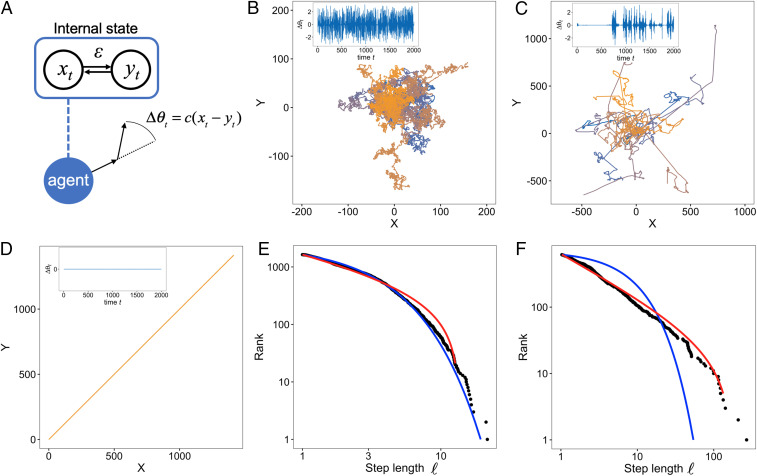
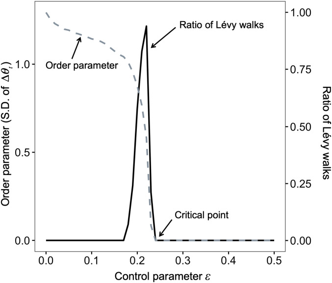
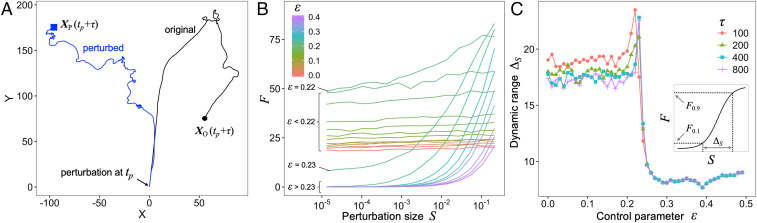
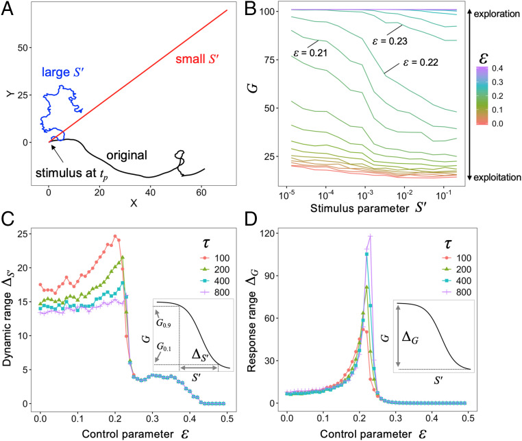
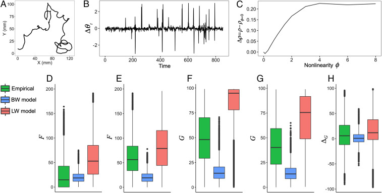
A special class of random walks, so-called Lévy walks, has been observed in a variety of organisms ranging from cells, insects, fishes, and birds to mammals, including humans. Although their prevalence is considered to be a consequence of natural selection for higher search efficiency, some findings suggest that Lévy walks might also be epiphenomena that arise from interactions with the environment. Therefore, why they are common in biological movements remains an open question. Based on some evidence that Lévy walks are spontaneously generated in the brain and the fact that power-law distributions in Lévy walks can emerge at a critical point, we hypothesized that the advantages of Lévy walks might be enhanced by criticality. However, the functional advantages of Lévy walks are poorly understood. Here, we modeled nonlinear systems for the generation of locomotion and showed that Lévy walks emerging near a critical point had optimal dynamic ranges for coding information. This discovery suggested that Lévy walks could change movement trajectories based on the magnitude of environmental stimuli. We then showed that the high flexibility of Lévy walks enabled switching exploitation/exploration based on the nature of external cues. Finally, we analyzed the movement trajectories of freely moving Drosophila larvae and showed empirically that the Lévy walks may emerge near a critical point and have large dynamic range and high flexibility. Our results suggest that the commonly observed Lévy walks emerge near a critical point and could be explained on the basis of these functional advantages.

Keywords: autonomous agent; criticality; movement ecology; nonlinear dynamics; random search.

Fig. 1.

Our model scheme and examples of trajectories and step length distributions obtained from the model. (A) The internal dynamics $x_t$ and $y_t$ produce the agent movements. The model has a parameter that determines the coupling strength between elements in the system. The movement is simply produced by turning angles $\mathrm{\Delta }{\theta }_t$. (B–D) The trajectory of the agent in a 2D space from $t=0$ to $\mathrm{2,000}$ is represented by solid lines: (B) $\epsilon =0.1$, (C) $\epsilon =0.22$, and (D) $\epsilon =0.3$. The different colors correspond to different initial conditions. Note that the trajectories in D are overlaid because they are exactly the same. The parameter of the tent map was set to $r=0.7$, and the initial position $\mathbf{X}\left(0\right)$ was set to (0, 0). Examples of the time series of the turning angle $\mathrm{\Delta }{\theta }_t$ are shown in Insets. When the value of $\mathrm{\Delta }{\theta }_t$ is close to zero for a long time, the agent exhibits straight movement. In contrast, when $\mathrm{\Delta }{\theta }_t$ fluctuates dynamically, the agent makes many turns. (E and F) Log–log plots of the rank distribution of step lengths $\ell$ in the trajectories obtained from the model for $\epsilon =0.1$ and $\epsilon =0.22$, respectively. Black dots represent the distribution of step length from the model movements as shown in B and C. The other parameters were set to $r=0.7$ and $t_{max}=\mathrm{10,000}$. The red and blue lines represent the fitted distribution of the truncated power-law and the exponential distribution, respectively.

Fig. 2.

Phase diagram with a changing control parameter $\epsilon$. The gray dashed line represents the order parameter, which is the SD of the distribution of $\mathrm{\Delta }{\theta }_t$. Near $\epsilon =0.22$, the order parameter changes drastically. The solid black line represents the ratio of the classification of Lévy walks obtained by fitting distributions to the simulated 100 trajectories for the same parameter set. The other parameters were set to $r=0.7$ and $t_{max}=\mathrm{10,000}$.

Fig. 3.

Dynamic range. (A) An example of trajectories for $\epsilon =0.22$ with (blue line) and without (black line) perturbations. We added a perturbation $S=10^{-4}$ to the internal dynamics of $x$ and $y$ only at $t_p$ and $\mathbf{X}\left(t_p\right)=\left(\mathrm{0,0}\right)$. The black circle and blue square represent the positions at $t=t_p+\tau$ (here $\tau =400$) of the original and perturbed trajectories, respectively. A trajectory change $F$ is defined as the distance between ${\mathbf{X}}_{\mathrm{O}}\left(t_p+\tau \right)$ and ${\mathbf{X}}_{\mathrm{P}}\left(t_p+\tau \right)$. (B) Relationship between perturbation size $S$ and $F$ for $\tau =100$. (C) Control parameter $\epsilon$ and dynamic range ${\mathrm{\Delta }}_S$. Inset represents the definition of dynamic range ${\mathrm{\Delta }}_S$. These results represent values averaged over $10^3$ simulation runs with different initial conditions.

Fig. 4.

Switching between exploitation and exploration. (A) An example of trajectories for $\epsilon =0.22$ with (red, $S^{\prime }=10^{-4}$; blue, $S^{\prime }=0.3$) and without (black) stimuli. The agents received the stimuli only at $t_p$ and $X\left(t_p\right)=\left(\mathrm{0,0}\right)$. We observed the position after $\tau$ (here $\tau =100$) and calculated the distance $G$ between $X\left(t_p\right)=\left(\mathrm{0,0}\right)$ and $X\left(t_p+\tau \right)$. (B) Relationship between stimuli parameters $S^{\prime }$ and $G$ for $\tau =100$. (C) Dynamic range ${\mathrm{\Delta }}_{S^{\prime }}$ and control parameter $\epsilon$. Inset represents the definition of ${\mathrm{\Delta }}_{S^{\prime }}$. (D) Response range ${\mathrm{\Delta }}_G$ and control parameter $\epsilon$. Inset represents the definition of ${\mathrm{\Delta }}_G$. These results represent values averaged over $10^3$ simulation runs with different initial conditions.

Fig. 5.

Empirical analysis. (A and B) Example of a movement trajectory of Drosophila larvae and the corresponding time series of turning angles, respectively. (C) Example of the result of S-map to check nonlinearity of the time series. (D–H) The results of perturbation analysis. (D and E) The corresponding cases of small and large $S$ for $\tau =100$, respectively. (F and G) The corresponding cases of small and large $S^{\prime }$ for $\tau =100$, respectively. (H) The difference of $G$ between F and G. Note that BW and LW model mean the proposed model with $\epsilon =0.0$ and 0.22, respectively. In D–H, all pairwise differences among the empirical, BW model, and LW model were statistically significant ($p<10^{-15}$). The black dots in D–H represent outliers, defined as data points outside the whiskers, which correspond to 1.5 times the interquartile range.

References

1. Viswanathan G. M., da Luz M. G. E., Raposo E. P., Stanley H. E., The Physics of Foraging: An Introduction to Random Searches and Biological Encounters (Cambridge University Press, 2011).
1. Harris T. H., et al. , Generalized Lévy walks and the role of chemokines in migration of effector CD8+ T cells. Nature 486, 545–548 (2012). - PMC - PubMed
1. Huda S., et al. , Lévy-like movement patterns of metastatic cancer cells revealed in microfabricated systems and implicated in vivo. Nat. Commun. 9, 4539 (2018). - PMC - PubMed
1. Humphries N. E., et al. , Environmental context explains lévy and brownian movement patterns of marine predators. Nature 465, 1066–1069 (2010). - PubMed
1. Raichlen D. A., et al. , Evidence of Lévy walk foraging patterns in human hunter–gatherers. Proc. Natl. Acad. Sci. U.S.A. 111, 728–733 (2014). - PMC - PubMed
Publication types
LinkOut - more resources