Dense neuronal reconstruction through X-ray holographic nano-tomography

Abstract

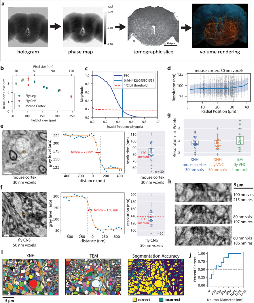
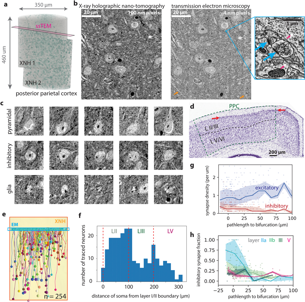
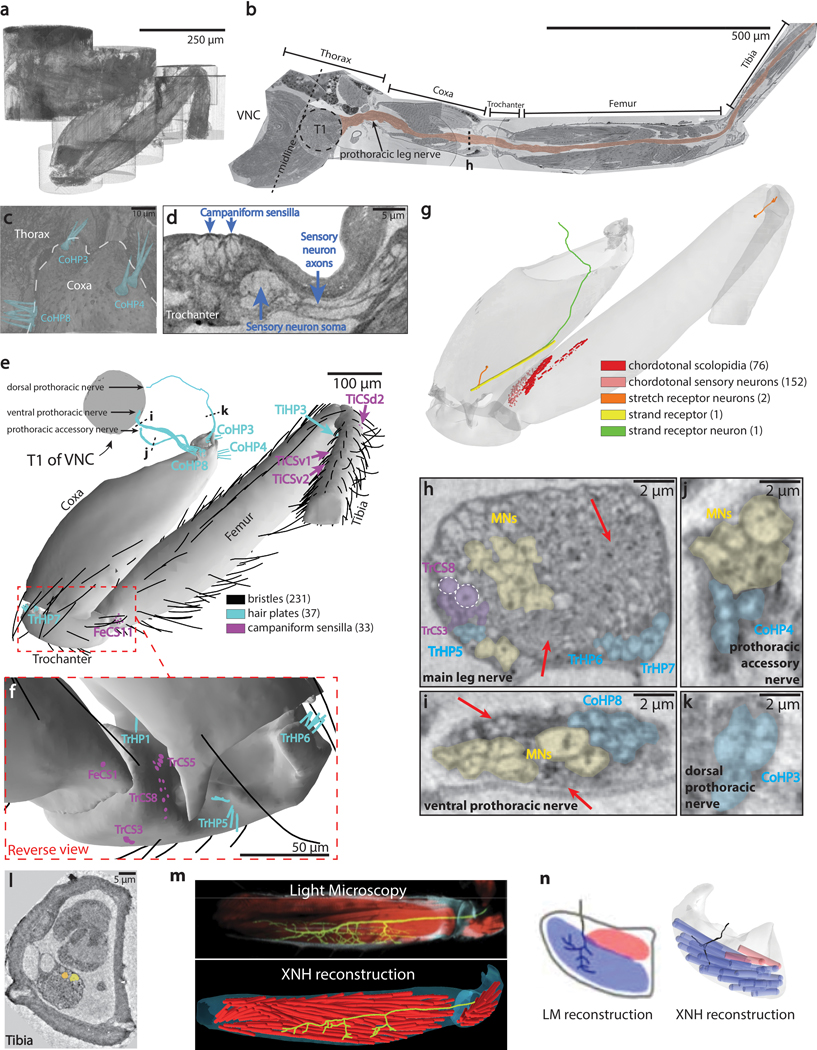
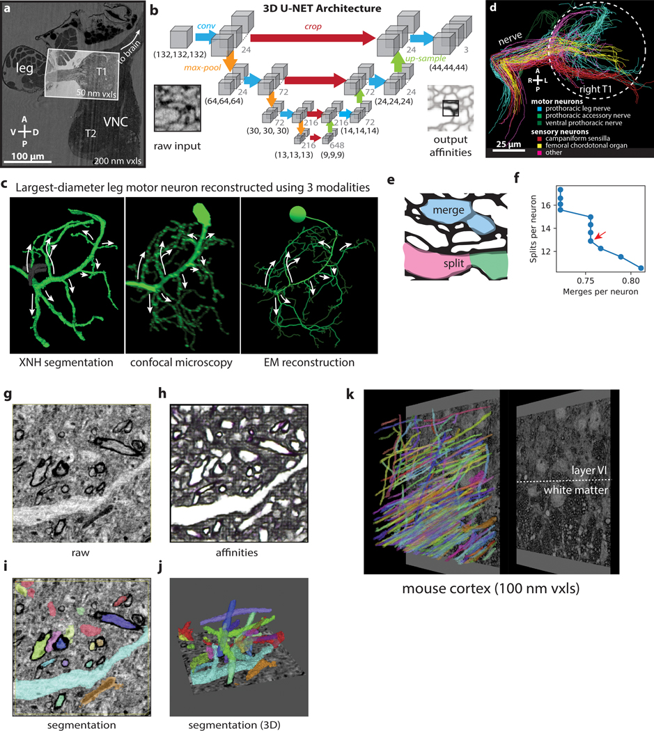
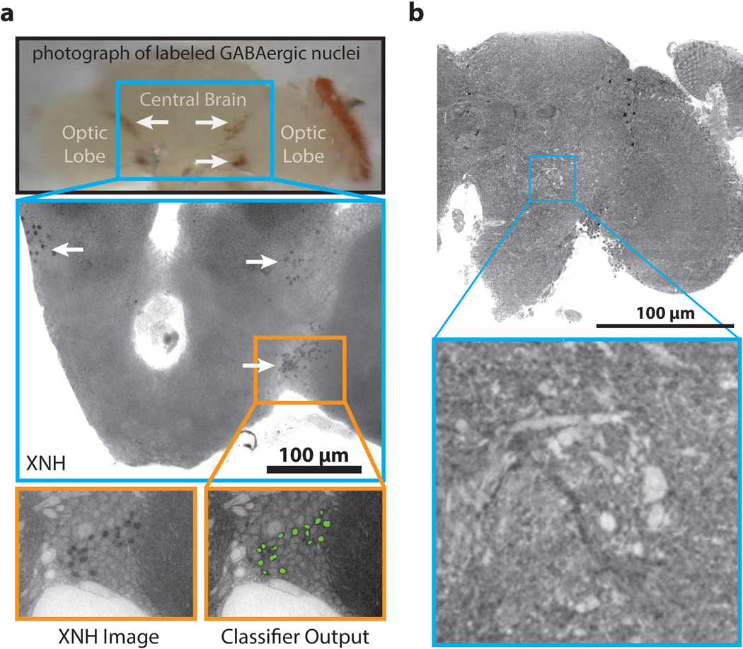
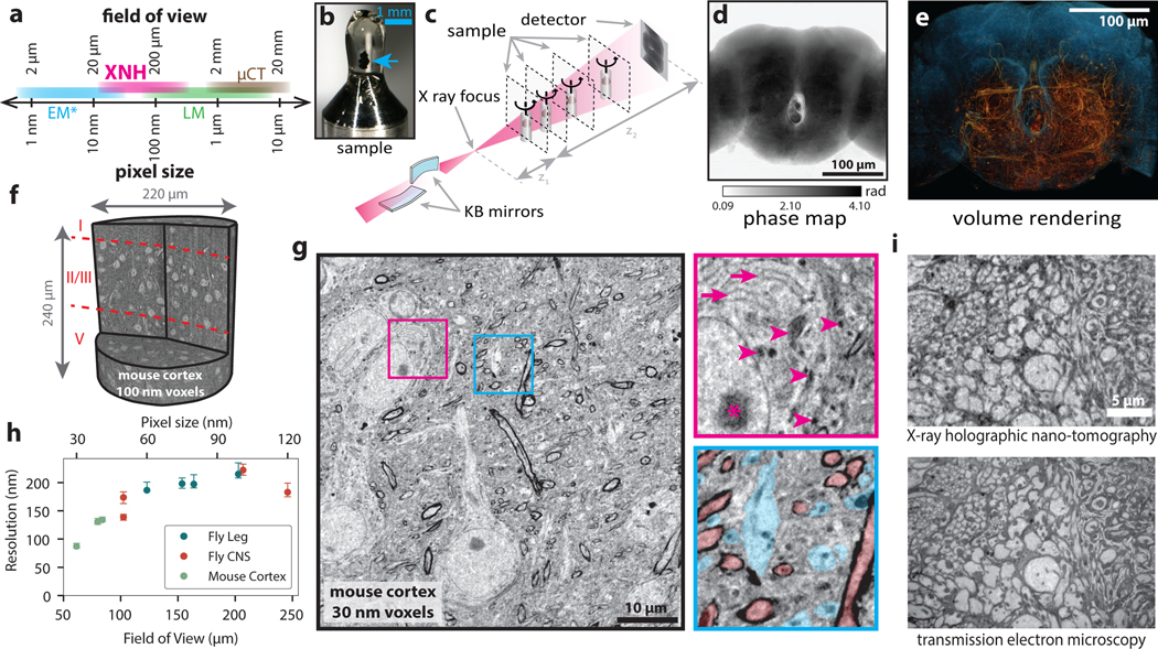
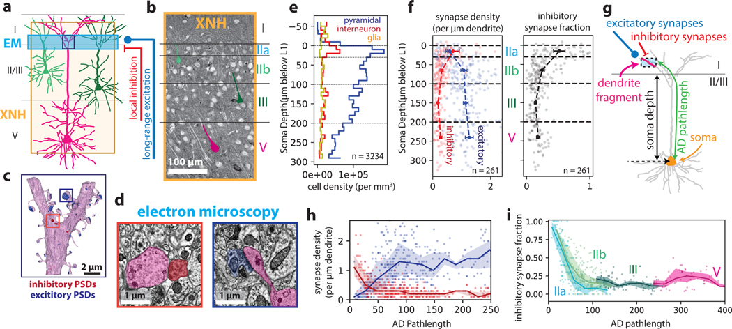
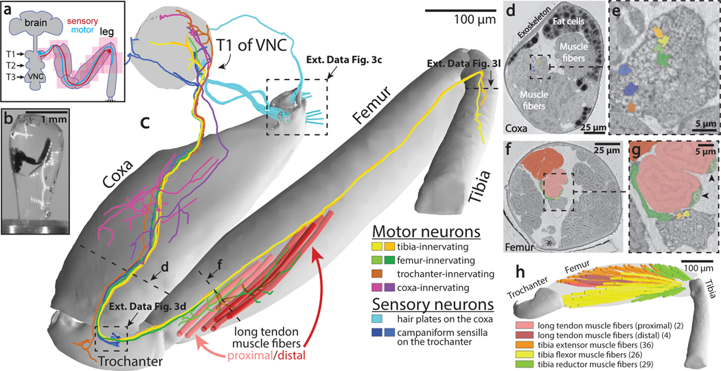
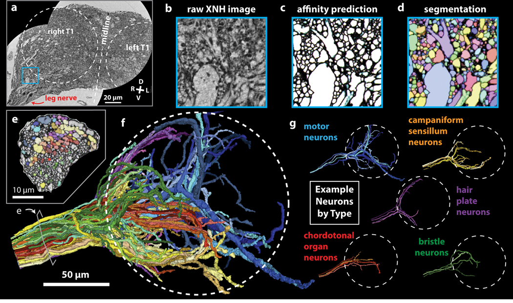
Imaging neuronal networks provides a foundation for understanding the nervous system, but resolving dense nanometer-scale structures over large volumes remains challenging for light microscopy (LM) and electron microscopy (EM). Here we show that X-ray holographic nano-tomography (XNH) can image millimeter-scale volumes with sub-100-nm resolution, enabling reconstruction of dense wiring in Drosophila melanogaster and mouse nervous tissue. We performed correlative XNH and EM to reconstruct hundreds of cortical pyramidal cells and show that more superficial cells receive stronger synaptic inhibition on their apical dendrites. By combining multiple XNH scans, we imaged an adult Drosophila leg with sufficient resolution to comprehensively catalog mechanosensory neurons and trace individual motor axons from muscles to the central nervous system. To accelerate neuronal reconstructions, we trained a convolutional neural network to automatically segment neurons from XNH volumes. Thus, XNH bridges a key gap between LM and EM, providing a new avenue for neural circuit discovery.

Extended Data Figure 1:. X-ray Holographic Nano-Tomography (XNH) Technique and Characterization.

(a) Overview of XNH imaging and preprocessing. Left: Holographic projections of the sample (a result of free-space propagation of the coherent X-ray beam) are recorded for each angle as the sample is rotated over 180°, then normalized with the incoming beam. Center left: Phase projections are calculated by computationally combining four normalized holograms recorded with the sample placed at different distances from the beam focus. Center right: Virtual slices through the 3D image volumes are calculated using tomographic reconstruction. Right: The resulting XNH image volume can be rendered in 3D and analyzed to reveal neuronal morphologies. (b) Quantification of resolution of XNH scans measured using Fourier Shell Correlation (FSC), normalized by each scan’s pixel size. At larger pixel sizes, the resolution per pixel improves, though the resolution itself is worse (see Fig. 1h). Datapoints and error bars show mean ± IQR of subvolumes sampled from each XNH scan. Number of subvolumes used for each scan is shown in Supplementary Data Table 1. (c) Representative FSC curve shown with the half-bit threshold. The intersection between the FSC curve and the threshold is the measured resolution. (d) Quantification of resolution within the 30 nm mouse cortex scan. Each dot represents an FSC measurement of a 100 voxel cube. Blue line and shaded band represent binned averages and standard deviation, respectively. The x-axis is the radial position of the center of the cube (distance from the axis of rotation). The red dotted line indicates the boundary of the scan – data points to the right of the line are from extended field of view regions (Methods). (e-f) Edge-fitting measurements of spatial resolution. Although FSC is commonly used to quantify resolution in many imaging modalities including X-ray imaging, its implementation is somewhat controversial. To ensure that FSC measurements were accurate, we also used an independent measure of resolution based on fitting sharp edges in the images (see Methods), which produced values consistent with those measured via FSC. Left: Example features used for edge-fitting resolution measurement. For both (e) mouse cortex and (f) fly central nervous system, mitochondria were primarily selected because they have dark contrast and sharp boundaries. Center: Example line scan (image intensity values along the orange lines in the feature images). The measured resolution is parameterized from a best-fit to a sigmoid function (Methods). Right: Distribution of edge-fitting resolution measurements for many features distributed throughout the image volumes. n = 30 features measured as shown; boxes shows median and IQR and whiskers show range excluding outliers beyond 1.5 IQR from the median. The median resolution measured via FSC is shown for comparison. (g) Comparison of edge-fitting resolution measurements for two XNH scans and high-resolution transmission EM images. EM data was acquired from a ~40 nm thick section of Drosophila VNC tissue, imaged with 4 nm pixels. Resolution is plotted in units of pixels. n = 30 features for each dataset; boxes shows median and IQR and whiskers show range excluding outliers beyond 1.5 IQR from the median. (h) Comparison of XNH images acquired from the same FOV in the same sample (fly leg) at different voxel sizes. Within this range, the resolution improves monotonically, but not linearly, with voxel size. (i) Comparison of XNH and EM segmentations. The XNH and EM images shown in Fig. 1i were independently segmented. Colored patches in the left two images represent different neurons in the segmentation. The EM segmentation was taken as ground truth, and the XNH segmentation for each neuron was evaluated. The right-most image shows correct and incorrectly segmented neurons. (j) Quantification of XNH segmentation accuracy. The proportion of correctly segmentation neurons is plotted as a function of neuron size. Neurons larger then 200 nm diameter were segmented correctly more than 50% of the time. Note that this analysis used only 2D image data – additional 3D information would likely improve performance. In addition to the size of the neurons, the membrane contrast is also an important factor in accurately segmenting neurons in XNH. In a few cases, membranes between two axons were not clearly visible in XNH, causing them to be erroneously merged (i). Motor neurons in the leg nerve were also challenging to segment because they contain complex glial wrappings that are not always clearly resolved in XNH (i, right size of images).

Extended Data Figure 2:. Correlative XNH - EM analysis of the connectivity statistics of pyramidal apical dendrites in posterior parietal cortex (PPC).

(a) 3D rendering of two aligned and stitched XNH datasets in mouse posterior parietal cortex. Cell somata are colored in green (based on voxel brightness). Magenta plane indicates location of serial EM dataset. (b) Aligned XNH virtual slice (left) and EM image (right) of the same region of cortical tissue (horizontal section). After XNH imaging and thin sectioning, the ultrastructure of the tissue remains well preserved, allowing identification of synapses (inset right, arrows). The EM images also showed small cracks (orange arrows) and bubbles (inset, pink arrows), which may have been caused by XNH imaging. (c) Examples of pyramidal neurons (top), inhibitory interneurons (middle) and glia (bottom) from the XNH data. Cells types were identified by classic ultrastructural features^,,. Pyramidal cells were identified by their prominent apical dendrites, while glia were identified from the relative lack of cytoplasm in the somata and the presence of multiple darkly stained chromatin bundles near the edges of the nuclei. Images are 40 × 40 μm virtual coronal slices (100 nm thick). (d) Histological slice of Nissl stained coronal section including posterior parietal cortex from the Allen Brain Atlas (http://atlas.brain-map.org/). Higher density of cells is evident at the top of layer II (consistent with Fig. 2e). (e) Rendering of cells included in connectivity analysis. Apical dendrites were traced in the XNH data (yellow) from somata (colored spheres) up to the layer I/II boundary where we collected an EM volume (cyan). Although the EM volume only contains short (< 50 μm) fragments of each AD, combining data across hundreds of neurons allowed us to map synaptic I/E balance over hundreds of micrometers of path length (Fig. 2h–i). (f) Histogram of locations (cortical depth) of traced cells used for analysis of synaptic inputs onto apical dendrites. (g) Synapse densities (excitatory in blue, inhibitory in red) plotted as a function of pathlength to the initial bifurcation (as opposed to cell soma in Fig. 2i–j). Each marker corresponds to one dendrite fragment 10 μm long. Lines and shaded areas indicate binned average (20 μm bins) and interquartile range (mean ± SE). (h) Inhibitory synapse fraction plotted as a function of pathlength to the initial bifurcation. Each marker corresponds to one dendrite fragment colored based on the soma type. Lines and shaded areas indicate binned average and interquartile range (mean ± SE) for each soma type individually.

Extended Data Fig. 3:. Millimeter-scale imaging of a Drosophila leg at single-neuron resolution.

(a) 3D rendering of the dataset after individual scans were stitched together to form a continuous volume. (b) The image volume was computationally unfolded (ImageJ) to reveal the entire 1.4mm length of the main leg nerve. (c) Volume rendering of the three hair plates that sense the thorax-coxa joint. The clusters are positioned differently within the joint, implying that they are sensitive to different joint angle ranges. (d) Cross-section through the group of eight campaniform sensilla on the trochanter, revealing the underlying sensory neurons and their axons (blue, see Fig. 3c). (e-g) Locations of sensory receptors in the leg. See also Supplementary Data Table 3. (e) Anterior view of external sensory structures. TiCSv1 and TiCSv2 are on the reverse (ventral) side of the tibia. (f) Posterior view of the trochanter, where large number of external mechanosensory structures reside. (g) Partially-transparent view of the leg revealing internal sensory structures (see Supplementary Data Table 3). Coxal stretch receptor: a previous report identified stretch receptor neurons in each of the distal leg segments (femur, tibia, and tarsus) that sense joint angles and are required for proper walking coordination. We identified a neuron in the coxa whose morphology is consistent with the other stretch receptors and was possibly missed previously due to incomplete fluorescent labeling. This demonstrates that each major joint in the fly leg, and not only the distal joints, are monitored by a single stretch receptor neuron. Coxal strand receptor: we identified a single strand receptor in the coxa, innervated by a single sensory axon for which no cell body was visible in the leg. Strand receptor neurons are unique sensory neurons that have a cell body in the VNC instead of the leg, but this type of neuron has only been previously identified in locusts and other orthopteran insects. In this reconstruction, the strand receptor neuron’s axon enters the VNC through the accessory nerve, but could not be reconstructed back to its cell body in the VNC. (h-k) Axons of some sensory neurons were large enough to reconstruct at the 150–200 nm resolution achieved here. Sensory neurons innervating coxal hair plates (cyan) and some trochanteral campaniform sensilla (blue) had axons with large diameters, similar in size to motor neuron axons (yellow). In contrast, axons of all chordotonal and bristle neurons were narrower. (h) Cross-section through the main leg nerve at the location indicated in (b). Axons from different sensory clusters bundle together. Two TrCS8 neurons have unusually large diameters (1050 nm and 850 nm, white circles; see Fig 3c for full reconstruction of these axons). The remaining TrCS neurons have axon diameters of 430 ± 140 nm. Motor neurons (yellow) have diameters of 1–2 μm. The unresolved axons (areas indicated by red arrows) are chordotonal neurons and bristle neurons. (i) Cross-section through the ventral prothoracic nerve at the location indicated in (e). Axons from CoHP8 sensory neurons (blue, axon diameters of 1030 ± 90 nm) travel in this nerve, which also contains seven motor neuron axons (yellow), five of which innervate muscles in the coxa (left, axon diameters of 1140 ± 130 nm), and two of which innervate muscles in the thorax (left, axon diameters of 1880 and 2150 nm). The unresolved axons (red arrows) are likely bristle neurons. (j) Cross-section through the prothoracic accessory nerve at the location indicated in (e). Axons from CoHP4 sensory neurons (cyan, axon diameters of 1140 ± 240 nm) travel in this nerve. Shown here is a cross-section through one of two major branches of the prothoracic accessory nerve. This branch also contains five motor neuron axons (yellow, axon diameters 1610 ± 240 nm). (k) Cross-section through the dorsal prothoracic nerve at the location indicated in (e). Axons from CoHP3 sensory neurons (cyan, axon diameters of 1380 ± 20 nm) enter the VNC through this nerve. Shown here is the branch of the dorsal prothoracic nerve containing only the CoHP3 axons. Panels (h-k) are slices through reconstructed XNH volumes with 75nm pixel size, subsequently Gaussian blurred with an 0.3 pixel radius. Axon diameters are reported as mean ± SD. (l) Cross-section through the tibia. The nerve is substantially smaller than in Fig. 3d–g as only a subset of leg neurons extend into the tibia. (m) Top: Morphology of a single motor neuron axon (green dye fill) innervating muscle fibers (red phalloidin stain ) in the femur (image from Azevedo et al.). Each fly has a single motor neuron with this recognizable morphology^,. Bottom: XNH reconstruction of a motor neuron axon having the same recognizable morphology as the neuron as shown in the top panel. Red cylinders represent individual muscle fibers. (n) Left: Morphology of the motor neuron LinB-Tr2 (image from Baek & Mann 2009⁴⁰, Copyright 1999 Society for Neuroscience). This motor neuron is born from Lineage B, the second largest lineage of motor neurons. Right: XNH reconstruction of motor neuron axon having the same recognizable morphology as the neuron shown in the left panel. The thin terminal branches were not resolved in the XNH reconstruction.

Extended Data Figure 4:. Automated Segmentation of Neuronal Morphologies using Convolutional Neural Networks (CNNs).

(a) Overview of XNH image volume encompassing the anterior half of the VNC and the first segment of a front leg of an adult Drosophila (200 nm voxels). A smaller, higher resolution (50 nm voxels) volume centered on the prothoracic (T1) neuromere of the VNC and including the initial segment of the leg nerve was used for automatic segmentation. (b) Schematic of U-NET CNN architecture used for automated segmentation (adapted from ). Each blue arrow represents two successive convolutions. (c) Morphological comparison of the motor neuron with the largest-diameter branches out of all front leg motor neurons, reconstructed from three different flies using different modalities. Arrows indicate the largest-diameter branches, which match well across the three reconstructions. Left: Reconstruction using automated segmentation of XNH images. Gray segment indicates a merge error that was corrected during proofreading (Methods). Middle: Reconstruction from LM images of a dye-filled motor neuron labeled by 81A07-Gal4. This motor neuron controls the tibia flexor muscle and produces the largest amount of force of any fly leg motor neuron yet identified. Adapted from Azevedo et al.. Right: Skeleton reconstruction from EM images. Adapted from Maniates-Selvin et al. (d) Population of 90 neurons used for evaluating segmentation error rates. Skeletons were categorized based on their morphologies (as in Fig. 4f) ^,,. White circle indicates the boundary of the T1 neuropil. A, anterior; P, posterior. (e) Examples of merge and split errors. True membrane locations are shown in black. Errors usually result from incorrect prediction of which voxels correspond to membranes. (f) Average error rates of segmentation for the 90 neurons shown in (f). Automated segmentation is parametrized by an agglomeration threshold amounts to a trade-off between split and merge errors. Data points indicate split and merge error rates for different agglomeration thresholds (Methods). The ideal segmentation minimizes the time needed to identify and fix split and merge errors during proofreading (red arrow). Merge error calculations based on comparisons to sparse manual tracing are likely an underestimate of the true number of merge errors. Note that the human-annotated, ground truth segmentation of XNH data excludes some areas where features are too small to resolve; thus these error metrics for XNH segmentation may not be directly comparable to what has been reported for EM. (g-j) Automated segmentation of XNH data in mouse cortex (primary somatosensory, layer 5, 30 nm voxels). (g) Raw data (h) Affinities (zyx corresponding to RGB colors). (i) selected segmentation labels corresponding to (e). (j) Selected 3D renderings of segmented neuron fragments. (k) Large FOV segmentation of myelinated axons in the white matter below mouse parietal cortex. Segmentation of such myelinated axons can enable tracing of long-range inputs between brain areas at single-cell resolution.

Extended Data Figure 5:. Additional staining approaches for XNH imaging.

(a) Top: Photograph of fly brain with GABAergic nuclei labeled with APEX2 (arrows). Middle: XNH images (120 nm pixels, 15 μm thick minimum intensity projection) of the same fly brain after heavy metal staining, showing clusters of dark, APEX2 labeled GABAergic cell nuclei (arrows). Bottom: XNH virtual slice (120 nm thick) and output from an automated Random Forest image classifier trained to detect labeled cells (green). (b) XNH data (105 nm voxels) of a Drosophila brain that did not undergo heavy metal staining. Even in unstained soft tissue, phase-contrast imaging provides enough signal that single neurons can still be resolved. FOV encompasses the optic lobe and half of the central brain. See Supplementary Video 6 and Methods.

Figure 1:. X-ray Holographic Nano-Tomography (XNH) Technique and Characterization.

(a) Schematic depicting pixel and FOV sizes for XNH imaging, along with comparisons to other modalities (assumes a 4 Mpixel detector). Note that EM imaging is generally performed on thin sections or surfaces, while XNH, LM, and micro computed tomography (μCT) can penetrate thicker tissue samples. (b) A Drosophila brain (blue arrow) embedded in resin and mounted for XNH imaging. (c) Imaging setup: the X-ray beam is focused to a spot using two Kirkpatrick-Baez mirrors and traverses the sample before hitting the detector. Holographic projections of the sample (a result of free-space propagation of the coherent X-ray beam) are recorded for each angle as the sample is rotated over 180° (see Extended Data Fig. 1a, Methods) (d) Phase map of the sample shown in Fig. 1b, calculated by computationally combining holograms recorded at 4 different distances from the beam focus. Computed pixel values indicate phase in radians. (e) 3D rendering of XNH volume of the central fly brain (120 nm voxels). The tissue outline is shown in blue, while neurons are highlighted in orange. (f) 3D rendering of an XNH volume of mouse posterior parietal cortex (100 nm voxels). Boundaries between cortical layers are shown in red. (g) Virtual slice through a higher-resolution XNH volume of mouse primary somatosensory cortex (30 nm voxels). Insets: detailed views showing ultrastructural features including mitochondria (magenta arrowheads), endoplasmic reticulum (magenta arrows), nucleolus (magenta asterisk), large dendrites (cyan) and myelinated axons (red). Insets are 10 μm in width. (h) Measured resolution (obtained using Fourier Shell Correlation, see Methods, Supplementary Table 1) for different XNH scans plotted as a function of voxel size and FOV. Datapoints and error bars show mean ± IQR of subvolumes sampled from each XNH scan. Number of subvolumes used for each scan is shown in Supplementary Data Table 1. (i) Comparison of XNH (50 nm voxels) and transmission electron microscopy (12 nm pixels, 100 nm section thickness) images of the same sample, the prothoracic leg nerve of an adult Drosophila.

Figure 2:. Correlative XNH - EM analysis of the connectivity statistics of pyramidal apical dendrites in posterior parietal cortex (PPC).

(a) Experimental approach: XNH imaging covers superficial and deep layers of PPC with sufficient resolution to resolve cell bodies and apical dendrites (ADs). Targeted 3D EM volume captures the layer I/II interface region, enabling analysis of synaptic inputs onto the apical dendrites near their initial bifurcations. (b) Virtual slice of XNH data (4 μm coronal section, max projection). Cell somata and apical dendrites are visible. Example layer II/III (green) and V (magenta) pyramidal cells are highlighted. (c) 3D EM reconstruction of an AD bifurcation with excitatory (targeting spines, blue) and inhibitory (targeting shafts or spine necks, red) synaptic inputs. (d) Example EM images of inhibitory (red) and excitatory (blue) synapses onto the apical dendrite. (e) Density of cell somata as a function of soma depth (μm below the layer I/II interface), classified as excitatory pyramidal cells (blue), inhibitory interneurons (red) or glia (yellow) (see Extended Data Fig. 2c). The top of layer II (~30 μm) contains a high density of both excitatory and inhibitory neurons. n = 3234 neurons. (f) Left: Synapse density plotted as a function of soma depth (μm below the layer I/II boundary). Excitatory and inhibitory synapses densities shown in blue and red, respectively. Right: Inhibitory synapse fraction plotted as a function of soma depth. Small markers correspond to one neuron. Large markers and error bars indicate mean and 95% confidence interval for each layer calculated via bootstrap analysis. n = 39, 99, 75, 38 neurons for layer IIa, IIb, III and V, respectively. (g) Schematic of dendrite-fragment connectivity analysis. Apical dendrites within the EM volume were divided into fragments 10 μm in length. For each fragment, the density of synapses was recorded along with the pathlength distance from the soma (AD pathlength). (h) Synapse densities (excitatory in blue, inhibitory in red) plotted as a function of pathlength to soma. Each marker corresponds to a 10 μm-long dendrite fragment. Lines and shaded areas indicate binned average (20 μm bins) and interquartile range. (i) Inhibitory synapse fraction plotted as a function of pathlength to soma. Each marker corresponds to one dendrite fragment, colored based on soma type. Lines and shaded areas indicate binned average and interquartile range (mean ± SE) for each soma type.

Figure 3:. Millimeter-scale imaging of a Drosophila leg at single-neuron resolution.

(a) Schematic of XNH imaging strategy. Ten partially-overlapping XNH scans (Supplementary Data Table 2) were used to capture a front leg’s coxa, trochanter, femur, and half of the tibia, plus the prothoracic neuromere (T1) of the VNC that controls this leg’s movements. The final leg segment, the tarsus, contains no muscles and was not imaged. (b) Photograph of a leg sample after heavy-metal staining, resin embedding, and mounting for XNH imaging. (c) Rendering of reconstructed leg segments, sensory neurons, motor neurons, and muscle fibers. Individual neurons were reconstructed from their target structures in the leg (sensory receptors or muscle fibers) into the VNC. (d-g) Cross-sections through the coxa and femur at locations indicated by dotted lines in (c). Color code is the same as in (c). (d) The arrangement of neurons, muscle fibers, and fat cells in the coxa. (e) Detailed view of nerve from (d). (f) The six long tendon muscle fibers in the femur are organized as a group of two and a group of four, which attach to the long tendon at different locations (see (c)). Asterisk indicates the femoral chordotonal organ, a proprioceptive sensory structure (see Extended Data Fig. 3g). (g) Detailed view of nerve from (f). Arrowheads indicate swellings of motor neuron axons, likely sites of neuromuscular junctions. Visible here are two swellings from the only motor neuron that innervates these two fibers (light green, see (c)). A different motor neuron (dark green, see (c)) branches off of the leg nerve, traveling past the proximal fibers to innervate the distal fibers. (h) Muscle fibers of the femur. The 97 fibers identified in the femur using XNH is nearly triple that reported previously using fluorescence microscopy.

Figure 4:. Automated Segmentation of Neuronal Morphologies using Convolutional Neural Networks (CNNs).

(a-b) Raw XNH image data, recorded from the T1 neuromeres of an adult Drosophila VNC. V, ventral; D, dorsal; R, right; L, left. (c) Predicted affinities output by a 3D U-NET (Extended Data Figure 4b) corresponding to the region shown in (b). The affinities quantify how likely it is that each voxel is part of the same neuron as neighboring voxels in z, y and x directions (plotted as RGB). In isotropic XNH data, affinities in different cardinal directions are usually similar, leading to images that appear mostly grayscale. The dark (low affinity) voxels are the basis for membrane predictions. (d) Segmentation corresponding to data shown in (b) and affinities shown in (c). Each neuron is agglomerated into a 3D morphology based on the affinities. In this visualization, each neuron has a unique color. (e) Cross-section of the main leg nerve showing motor and sensory axons reconstructed via automated segmentation. Coloring corresponds to neuron type, revealing spatial organization of neurons within the nerve. (f) 3D visualization of 100 automatically segmented neurons in the Drosophila VNC. Coloring corresponds to neuron types determined based on 3D morphology. Dotted circle indicates boundary of the T1 neuropil associated with control of the front leg. (g) Example morphologies of VNC neuron subclasses (only four example neurons per type shown for clarity).

References

1. Denk W, Briggman KL & Helmstaedter M. Structural neurobiology: missing link to a mechanistic understanding of neural computation. Nat. Rev. Neurosci. 13, 351–8 (2012). - PubMed
1. Xu CS et al.Enhanced FIB-SEM systems for large-volume 3D imaging. Elife 6, (2017). - PMC - PubMed
1. Lee W-CA et al.Anatomy and function of an excitatory network in the visual cortex. Nature 532, 1–18 (2016). - PMC - PubMed
1. Zheng Z. et al.A Complete Electron Microscopy Volume of the Brain of Adult Drosophila melanogaster. Cell 174, 730–743.e22 (2018). - PMC - PubMed
1. Hell SW Far-field optical nanoscopy. Science 316, 1153–8 (2007). - PubMed
Methods References
1. Hua Y, Laserstein P. & Helmstaedter M. Large-volume en-bloc staining for electron microscopy-based connectomics. Nat. Commun. 6, 7923 (2015). - PMC - PubMed
1. Zhang Q, Lee W-CA, Paul DL & Ginty DD Multiplexed peroxidase-based electron microscopy labeling enables simultaneous visualization of multiple cell types. Nat. Neurosci. 22, 828–839 (2019). - PMC - PubMed
1. Du M. & Jacobsen C. Relative merits and limiting factors for x-ray and electron microscopy of thick, hydrated organic materials. Ultramicroscopy 184, 293–309 (2018). - PMC - PubMed
1. Lam SS et al.Directed evolution of APEX2 for electron microscopy and proximity labeling. Nat. Methods 12, 51–54 (2015). - PMC - PubMed
1. Berg S. et al.ilastik: interactive machine learning for (bio)image analysis. Nat. Methods (2019) doi:10.1038/s41592-019-0582-9. - DOI - PubMed
Extended Data References
1. . Hodgkin HM & Bryant PJ Scanning electron microscopy of the adult of Drosophila melanogaster. Genet. Biol. Drosoph. (1979).
1. . Court RC et al. A Systematic Nomenclature for the Drosophila Ventral Nervous System. bioRxiv 122952 (2017) doi:10.1101/122952. - DOI
Publication types