A comparison of neuronal population dynamics measured with calcium imaging and electrophysiology

Abstract

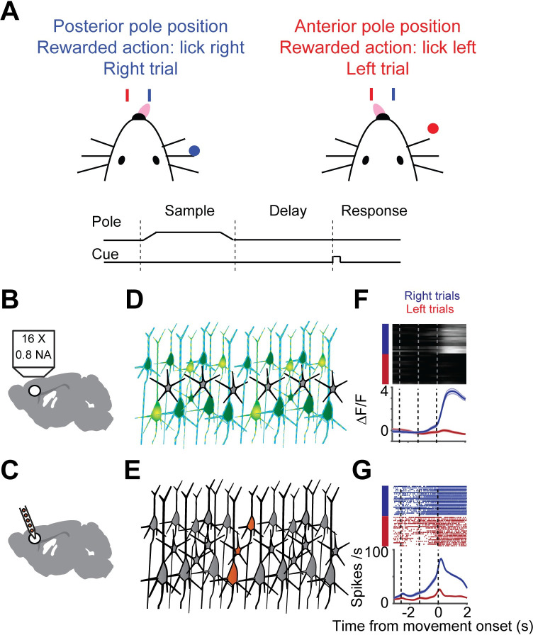
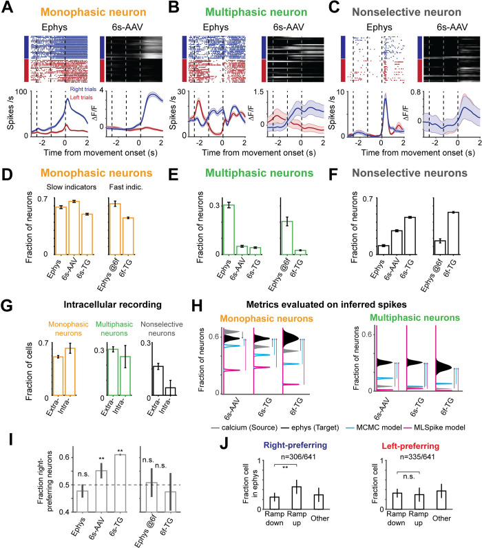
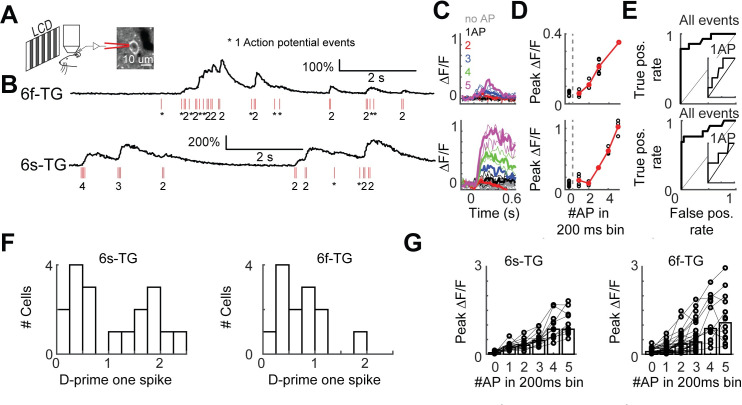
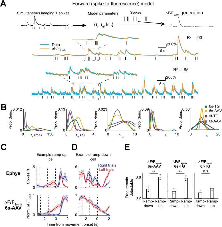
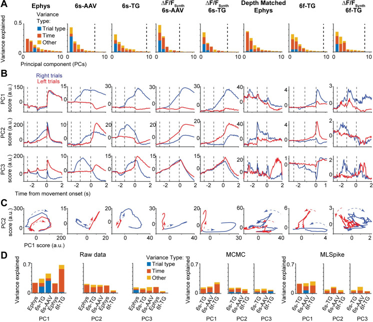
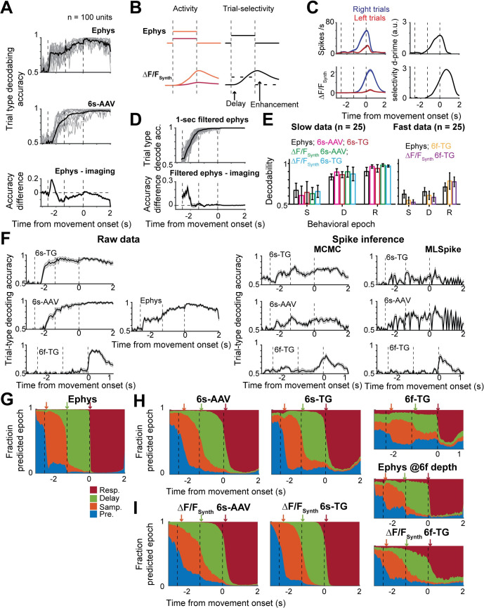
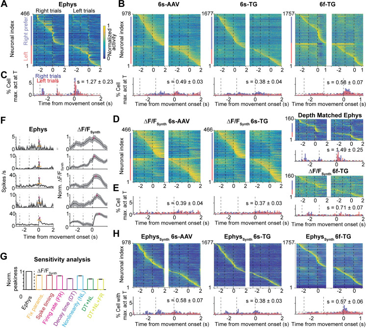
Calcium imaging with fluorescent protein sensors is widely used to record activity in neuronal populations. The transform between neural activity and calcium-related fluorescence involves nonlinearities and low-pass filtering, but the effects of the transformation on analyses of neural populations are not well understood. We compared neuronal spikes and fluorescence in matched neural populations in behaving mice. We report multiple discrepancies between analyses performed on the two types of data, including changes in single-neuron selectivity and population decoding. These were only partially resolved by spike inference algorithms applied to fluorescence. To model the relation between spiking and fluorescence we simultaneously recorded spikes and fluorescence from individual neurons. Using these recordings we developed a model transforming spike trains to synthetic-imaging data. The model recapitulated the differences in analyses. Our analysis highlights challenges in relating electrophysiology and imaging data, and suggests forward modeling as an effective way to understand differences between these data.

Fig 1. Illustration of sampling population activity in anterior lateral motor cortex using imaging and electrophysiology.

A. Delayed-response, two alternative forced-choice task. Mice discriminated a pole position (anterior or posterior) and reported it by directional licking (lick right, blue; lick left, red) after a delay period. End of delay period was signaled by an auditory cue B. Schematic of imaging setup. C. Schematic of electrophysiological setup. D. Schematic of neurons sampled by imaging (green). E. Schematic of sampled neurons by electrophysiology (orange). F. Example neuron, imaging. Top, individual trials (blue, right trial; red, left trial). Bottom, mean activity (mean, thick line; sem., shaded area). G. Example neuron, electrophysiology. Top, raster plot. Bottom, peri-stimulus time histogram (PSTH).

Fig 2. Single neuron trial-type selectivity differs between imaging and ephys.

A. Example neurons with monophasic selectivity. Left, ephys; right, imaging. B, Same as A for multiphasic neurons. C, Same as A for non-selective neurons. D-F, Fraction of selective neurons in depth-matched ephys (“ephys @6f” indicates depth matched to the more superficial 6f-TG recordings) and when imaged with 6s-AAV, 6s-TG, or 6f-TG. D. Fractions of monophasic neurons. E. Fraction of multiphasic neurons. F. Fraction of nonselective G. Proportion of multiphasic neurons in intracellular recordings is similar to that in extracellular recordings. Bar shows fraction of neurons in each of the categories for extracellular (left) and intracellular (right) ephys. H. Effect of spike inference on estimates of fractions of monophasic (left) and multiphasic (right) neurons. The distribution of fraction of neurons for imaging data (source data), is given in gray for 6s-AAV (top), 6s-TG (middle) and 6f-TG (bottom). The distribution for ephys (target data) is in black. Distributions from inferred spike rates from MCMC (40) are in cyan and for MLSpike (42) are in magenta. Arrows denote the difference between the imaging data and ephys data (gray arrow) or inferred ephys and ephys data (cyan arrow for MCMC and magenta arrow for MLSpike). I. Fraction of right-preferring neurons in the different datasets divided into slow indicators (left) and fast indicators (right). J. Bar plot of fractions of ramp-down, ramp-up and ‘other’ cells in ephys for right-preferring (left) and left-preferring neurons (right).

Fig 3. Simultaneous loose-seal recordings and calcium imaging of layer 2/3 pyramidal neurons in vivo.

A. Illustration of the recording setup. Transgenic mice expressing GCaMP6s (GP4.3) or GCaMP6f (GP5.17) were lightly anesthetized and viewed drifting grating visual stimuli. GCaMP-expressing L2/3 neurons were recorded in the loose-seal mode during calcium imaging. B. Example recordings from neurons expressing GCaMP6f (top, 6f-TG) and GCaMP6s (bottom, 6s-TG). Red ticks, spikes. C. Traces of fluorescence dynamics following different numbers of action potentials (APs) for example neurons. Top, 6f-TG; bottom, 6s-TG. Gray, no AP; black, a single AP; red, 2 APs; blue, 3APs; green, 4APs; magenta, 5APs. Thin lines, single trials; thick lines, average. D. Peak fluorescence increases as a function of the number of spikes in 200 ms bins. Black, single trials; red, trial average. E. ROC curve of all spike events. Inner panel, ROC curve for single AP events. F. Distribution of d-prime for single spikes across cells. Left, 6s-TG; right, 6f-TG. G. Mean peak fluorescence changes as a function of number of spikes in 200 ms time intervals across cells. Left, 6s-TG; right, 6f-TG. Each circle corresponds to a recorded neuron. Bars indicate average.

Fig 4. Forward modeling of the spike-to-fluorescence transformation largely explains difference in selectivity patterns.

A. spike-to-fluorescence model. Top: schematic plot of the spike-to-fluorescence (S2F) forward model that generates a synthetic fluorescence trace (ΔF/F_Synth) from an input spike train. Middle: example fit and data of two cells. Experimental, measured ΔF/F (blue) is overlaid with the simulated ΔF/F_Synth (orange) from the S2F model. The input to the model, the simultaneously recorded spikes (black), is shown below the traces. B. Distributions of the inferred model parameters for different indicators (yellow: 6s-AAV; green: 6s-TG; Purple: 6f-TG; gray: 6f-AAV. C. An example ramp-up neuron (top, ephys; bottom, 6s-AAV synthetic of that neuron); selectivity remains detectable in synthetic imaging data. D. An example ramp-down neuron (top, ephys; bottom, 6s-AAV synthetic of that neuron); selectivity becomes undetectable in synthetic imaging. E. S2F model predicts that selectivity of ramp-down neurons but not ramp-up neurons, would be often obscured in imaging datasets. Bar plot shows fraction of cells that remain detectably selective in synthetic imaging (6s-AAV synthetic, left; 6s-TG synthetic, middle; 6f-TG synthetic, right) plotted separately for ramp-down and ramp-up cells.

Fig 5. Different sources of variability extracted in dimensionality reduction on imaging and ephys.

A. Fraction of variance of neural activity explained by principal components 1–10 divided into different sources of variability: red: temporal dynamics; blue: trial type; yellow: other (interaction term). From left to right: ephys, 6s-AAV, 6s-TG, 6s-AAV synthetic, 6s-TG synthetic; ephys depth-matched to 6f-TG recordings, 6f-TG, 6f-TG synthetic. Vertical dashed line indicates the PC index at which the remaining components capture <1% of total variance. B. Trial-averaged scores of first three PCs over time (from top to bottom), averaged separately for the two trial types (right trial, blue; left trial, red). Same order from left to right as in A. C. Trial dynamics in the first two-PC subspace for the two trial types (right trial, blue; left trial, red). Same order from left to right as in A. D. Left: fraction of variance explained by principal components 1–3 for each of the datasets, and its division into different sources of variability: red: temporal dynamics; blue: trial type; yellow: other (interaction term). Bars from left to right: ephys, 6s-TG, 6s-AAV; ephys depth-matched to 6f-TG recordings, 6f-TG. Middle: equivalent results for principal component analysis performed on inferred spiking data obtained via the MCMC framework. Right: equivalent results for principal component analysis performed on inferred spiking data obtained via the MLSpike framework.

Fig 6. Population decoding differs in sensitivity and temporal profile between imaging and ephys.

A. Performance of instantaneous regularized linear-discriminant-analysis (LDA) trail-type decoder for 100-unit subpopulations. Vertical dotted lines indicate behavioral epochs, from left to right: presample, sample, delay, response. Top, decoders trained on ephys; middle, decoders trained on 6s-AAV; bottom, difference between the two. For top and bottom plots: individual gray lines show single subsample performance and black thick line shows average. In bottom plot mean is indicated by think line and shaded area corresponds to standard deviation. B. Toy model demonstrating observed delayed but enhanced decodability in imaging data. Schematic of relation between activity (left) and decodability (right) when the model has two constant levels of activation for the two trial types (orange and red). C. Example cell showing similar behavior to the toy model. D. Comparison of decodability from imaging to decodability from 1-second filtered ephys. Top, 1-second filtered ephys; bottom, difference between filtered ephys and imaging. E. Comparison of decodability of trial type per behavioral epoch. Decodability for all datasets separated into slow indicators (left) and fast indicators (right). Bars color coded according to dataset. Left: black, ephys; magenta, 6s-AAV; red, 6s-TG; green, 6s-AAV synthetic; cyan, 6s-TG synthetic. Right: black, ephys (depth matched to 6f-TG); orange, 6f-TG; purple, 6f-TG synthetic. F. Accuracy of trial-type population decoding over time for different datasets. Left, top to bottom: 6s-TG, 6s-AAV, 6f-TG. Middle: ephys. Right, accuracy of trial-type population decoding over time of datasets comprised of inferred ephys from the different imaging datasets. top to bottom: 6s-TG, 6s-AAV, 6f-TG. Left column: MCMC framework, right column: MLSpike framework. G-I. Performance of behavioral-epoch LDA decoders. G. Probability of decoder based on ephys to assign population activity to each of the different epochs shown in the following color scheme: pre-sample (blue), sample (orange), delay (green), and response (red) epoch; arrows indicate the inferred transition times of epochs from neural codes. H. Same plot format as G, but for imaging. I. Sample plot format as G, but for synthetic imaging.

Fig 7. Temporal dispersion of population dynamics differs between imaging and ephys.

A. Heatmap of normalized trial-averaged firing rates for right trials (left) and left trials (right) for ephys data. Firing rates were normalized to maximum of activity across both conditions. Neurons were first divided into two groups by their preferred trial type then sorted by latency of peak activity. B. Same plots as A but for 6s-AAV (left), 6s-TG (middle) and 6f-TG (right). Below the 6f-TG are neurons from ephys depth matched to 6f-TG. C. Fraction of neurons with a peak at given time point over time. Distribution in time plotted simultaneously for both trial types (red: right trials, blue: left trials, black horizontal line: uniform distribution). Datasets shown left to right (from left: ephys, 6s-AAV, 6s-TG, and 6f-TG respectively). D-E. The same plots as B-C for synthetic imaging (6s-AAV synthetic, left; 6s-TG synthetic, middle; 6f-TG synthetic, right). F. Example cells with peaks at a similar time in ephys (left; mean activity, thick black line; sem, shaded area; peak, magenta circle; baseline, orange thin line) along with the corresponding synthetic data (right). Neurons are sorted according to their peak times in synthetic imaging (early to late, from top to bottom). G. Sensitivity analysis of peakiness by synthetic, artificial data (Materials and Methods). Bars show normalized peakiness for the different model variants: (1) identical S2F parameters and identical spike times; (2) identical S2F parameters, jittered spike times (3) identical S2F parameters, variable firing rate (4) identical S2F parameters except for the decay time constant of the calcium indicator that was randomly sampled from its distribution; (5) identical S2F parameters, except for the nonlinearity of the calcium indicator that was randomly sampled from its distribution; (6) both decay time constant and nonlinearity of calcium indicator randomly sampled; (7) variable decay time constant, non-linearity and firing rates. H. Same plots as B-C for inferred firing rates from imaging, i.e., synthetic ephys.

References

1. Buzsaki G. Large-scale recording of neuronal ensembles. Nat Neurosci. 2004;7(5):446–51. 10.1038/nn1233 - DOI - PubMed
1. Dhawale AK, Poddar R, Wolff SBE, Normand VA, Kopelowitz E, Ölveczky BP. Automated long-term recording and analysis of neural activity in behaving animals. eLife. 2017;6:e27702 10.7554/eLife.27702 - DOI - PMC - PubMed
1. Ganguly K, Carmena JM. Emergence of a stable cortical map for neuroprosthetic control. PLoS biology. 2009;7(7):e1000153 10.1371/journal.pbio.1000153 - DOI - PMC - PubMed
1. Tolias AS, Ecker AS, Siapas AG, Hoenselaar A, Keliris GA, Logothetis NK. Recording chronically from the same neurons in awake, behaving primates. J Neurophysiol. 2007;98(6):3780–90. 10.1152/jn.00260.2007 - DOI - PubMed
1. Peron SP, Freeman J, Iyer V, Guo C, Svoboda K. A Cellular Resolution Map of Barrel Cortex Activity during Tactile Behavior. Neuron. 2015;86(3):783–99. 10.1016/j.neuron.2015.03.027 - DOI - PubMed
Publication types