Analysis of temporal correlation in heart rate variability through maximum entropy principle in a minimal pairwise glassy model

Abstract

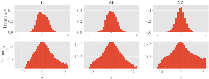
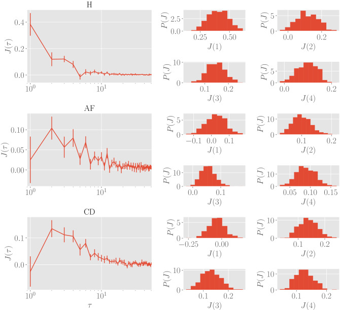
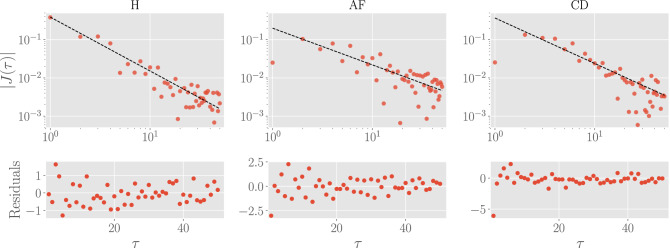
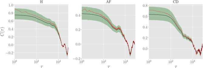
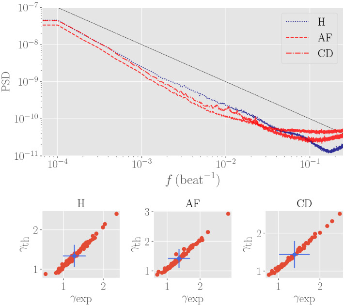
In this work we apply statistical mechanics tools to infer cardiac pathologies over a sample of M patients whose heart rate variability has been recorded via 24 h Holter device and that are divided in different classes according to their clinical status (providing a repository of labelled data). Considering the set of inter-beat interval sequences [Formula: see text], with [Formula: see text], we estimate their probability distribution [Formula: see text] exploiting the maximum entropy principle. By setting constraints on the first and on the second moment we obtain an effective pairwise [Formula: see text] model, whose parameters are shown to depend on the clinical status of the patient. In order to check this framework, we generate synthetic data from our model and we show that their distribution is in excellent agreement with the one obtained from experimental data. Further, our model can be related to a one-dimensional spin-glass with quenched long-range couplings decaying with the spin-spin distance as a power-law. This allows us to speculate that the 1/f noise typical of heart-rate variability may stem from the interplay between the parasympathetic and orthosympathetic systems.

Figure 1

Left: examples of the bare RR time series for a single patient for each class; the window depicted is restricted to the first 2000 beats. Right: examples of autocorrelation functions for a single patient for each class. The dotted blue line refers to a healthy patients, while red are patients with AF (dashed curve) and CD (dash-dotted line). Notice that, in any case, the autocorrelation remains positive over several orders of magnitude and this is a consequence of the scale-free behavior of the series power spectral density (see also Fig. 7, upper panel).

Figure 2

Histograms of the standardized values $\{\mathbf{z}(i)\}$ divided by classes: left panels are build by collecting data from healthy patients, middle panels are build by collecting data from patients suffering from atrial fibrillation and right panels are build by collecting data from patients suffering from cardiac decompensation. In the first row, we reported relative frequencies in the natural scale, while the second row we reported relative frequencies in the logarithmic scale.

Figure 3

Inference results for delayed interactions. Left column: the plots show the results of the inference procedure (distinguishing between the clinical status) for the first 50 $\tau$s. Right: frequency distribution of the Js for some selected values of $\tau$ (i.e. $\tau =1,2,3,4$). In both cases,the statistics consists in $M=500$ different realizations of the $J(\tau )$ which are realized by randomly extracting different mini-batches, each with size $n=20$. We stress that some frequency distributions present tails on negative values of J for some $\tau$. This means that frustrated interactions are also allowed, implying that the system is fundamentally complex, i.e. a glassy hearth.

Figure 4

Leading behavior of magnitude of the delayed interactions. In the upper panel, we reported the absolute value of the delayed interactions $J(\tau )$ and the relative best fit. In the lower panel, we reported the residuals (normalized by the uncertainty at each point $\tau$) of the experimental data with respect to the best fit function. We stress that, even if the interactions $J(\tau )$ are far from the fitting curve (in the log-log scale, see first row), they are compatible within the associated uncertainties, as remarked by the residual plots.

Figure 5

Comparison between posterior distributions for experimental and synthetic data. First row: comparisons between the empirical cumulative distributions for both experimental (solid red lines) and resampled (black dashed lines) populations for all of the three classes. Second row: probability plots for the two populations of data (i.e. empirical versus theoretical ones, red solid lines) for all of the three classes. The black solid curves are the identity lines for reference. The green region is the confidence interval with $p=0.95$.

Figure 6

Comparison between autocorrelation functions for experimental and synthetic data. The autocorrelation function for one patient randomly extracted from the experimental data-set (red solid lines) is compared with the median autocorrelation function obtained from the synthetic dataset (black dashed lines). Notice that the former falls in the confidence interval with $p=0.68$ (green region) of the latter.

Figure 7

Top: empirical power spectral density (PSD). The dotted blue line refers to a healthy patients, while the red ones refer to patients with AF (dashed curve) and CD (dash-dotted line). The PSD is computed according to the Welch procedure with $50\%$ windows overlap. The black continuous curve is the expected 1/f-noise distribution for visual comparison. Bottom: scatter plot for the scaling exponent of the PSD (in the region ${10}^{-4}$ e ${10}^{-2}$ Hz); in particular, we take the simple average over the synthetic realizations, the red spots are the exponent for the single patient (notice that the uncertainties over the synthetic realization are much smaller and are not visible in the plot), and the blue spot marks the average over all patients (both experimental and synthetic) with the relative uncertainties.

References

1. Agliari, E. et al., Detecting cardiac pathologies via machine learning on the clinical markers based on heart rate variability. Sci. Rep. 10, 8845 (2020). - PMC - PubMed
1. Barra, O.A. & Moretti, L., The “Life Potential” a new complex algorithm to assess “heart rate variability” from Holter records for cognitive and dignostic aims, avaiable atarXiv:1310.7230, (2013).
1. Jaynes ET. Probability theory: The logic of science. Cambridge: Cambridge University Press; 2003.
1. Sakellariou J, Tria F, Loreto V, Pachet F. Maximum entropy models capture melodic styles. Sci. Rep. 2017;7:9172–9185. - PMC - PubMed
1. Tkacik G, et al. The simplest maximum entropy model for collective behavior in a neural network. JSTAT. 2013;2013(03):3011–3043.
Publication types