Differential Emergence and Stability of Sensory and Temporal Representations in Context-Specific Hippocampal Sequences

Abstract

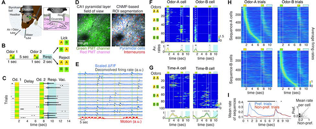
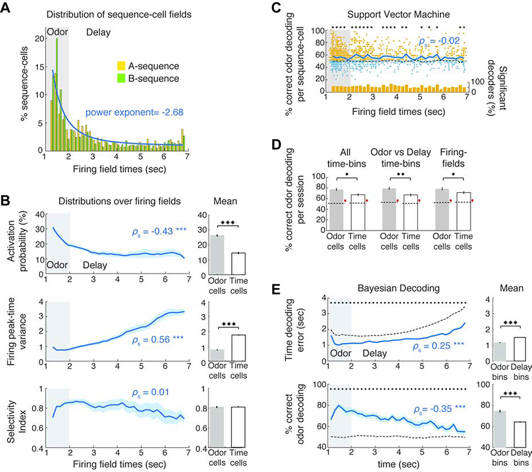
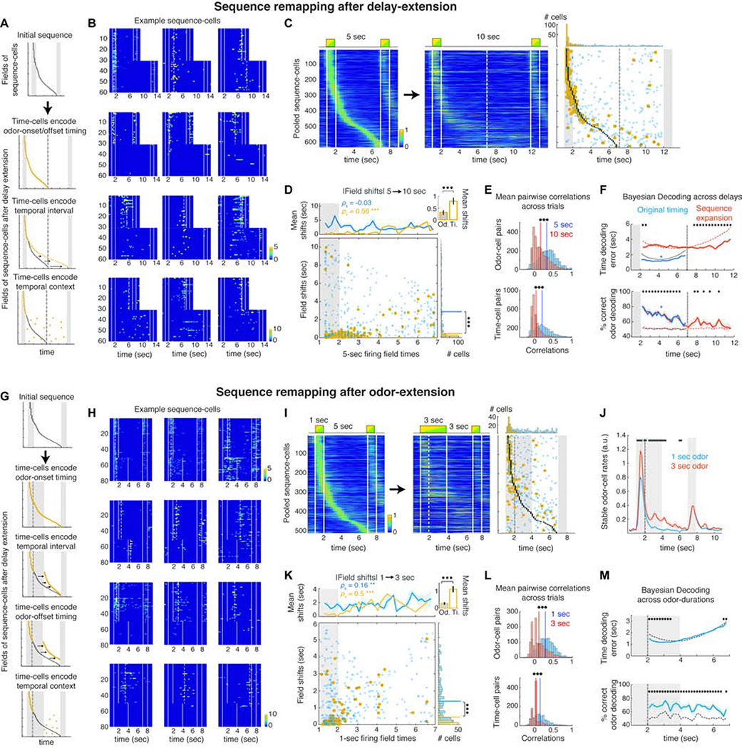
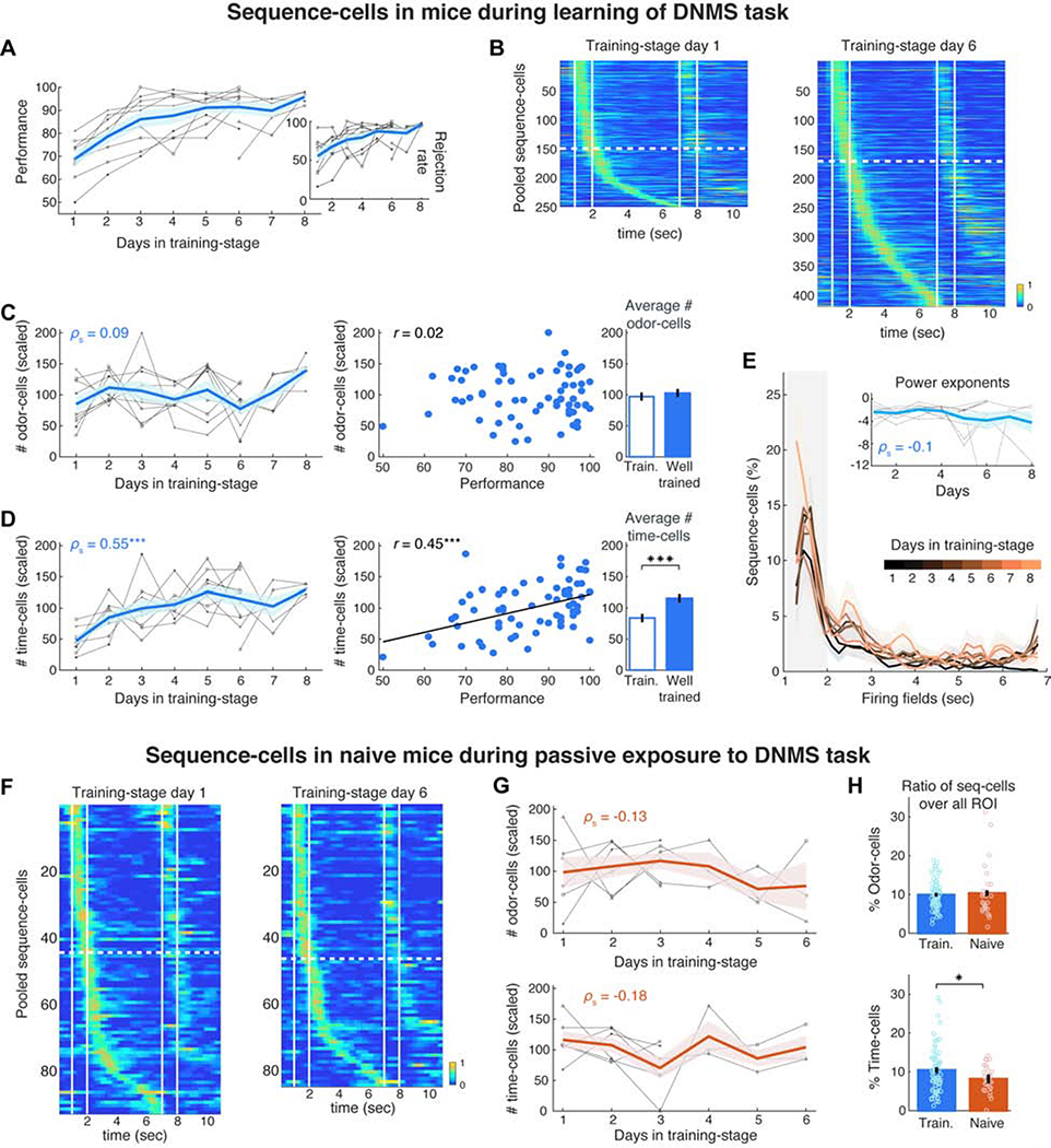
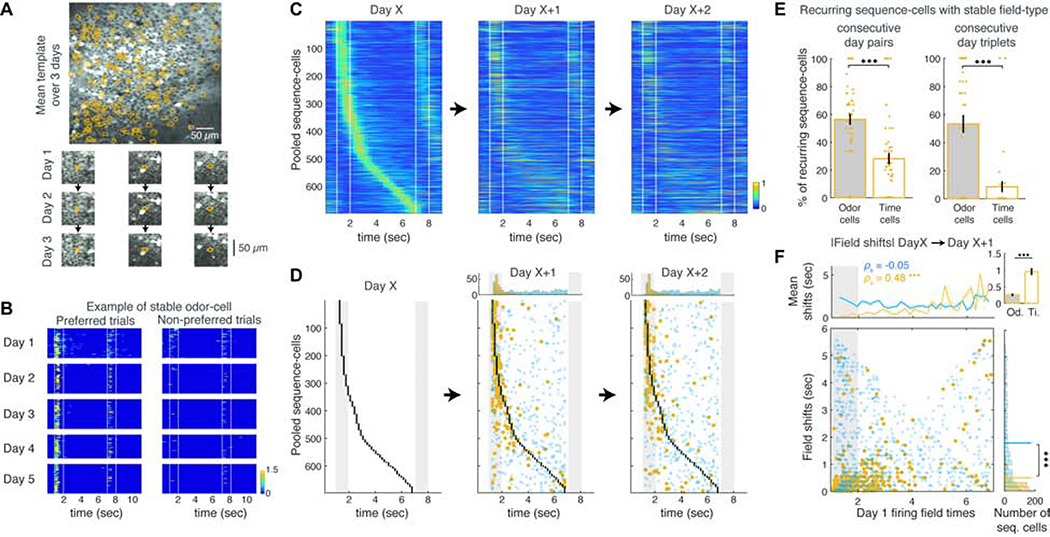
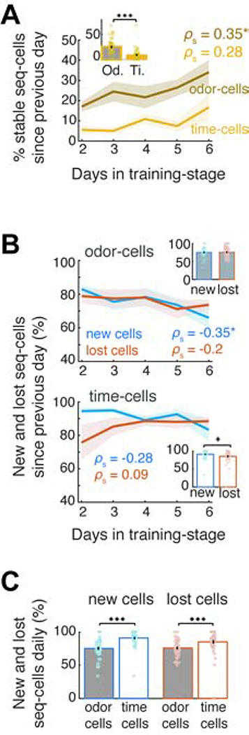
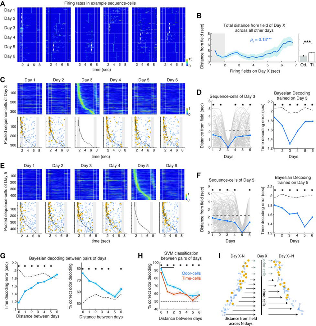
Hippocampal spiking sequences encode external stimuli and spatiotemporal intervals, linking sequential experiences in memory, but the dynamics controlling the emergence and stability of such diverse representations remain unclear. Using two-photon calcium imaging in CA1 while mice performed an olfactory working-memory task, we recorded stimulus-specific sequences of "odor-cells" encoding olfactory stimuli followed by "time-cells" encoding time points in the ensuing delay. Odor-cells were reliably activated and retained stable fields during changes in trial structure and across days. Time-cells exhibited sparse and dynamic fields that remapped in both cases. During task training, but not in untrained task exposure, time-cell ensembles increased in size, whereas odor-cell numbers remained stable. Over days, sequences drifted to new populations with cell activity progressively converging to a field and then diverging from it. Therefore, CA1 employs distinct regimes to encode external cues versus their variable temporal relationships, which may be necessary to construct maps of sequential experiences.

Keywords: CA1; Hippocampus; calcium imaging; drift; learning; odor; population dynamics; sequences; stability; time.

Figure 1:. Odor-specific spiking sequences in dCA1 encode cues and delay time in a DNMS task.

A. Behavioral and experimental set-up. CC: corpus callosum. B. Schematic of the DNMS trial. Licking is assessed during a 2 sec response window (blue). C. Example trial-block. Dots indicate licks. The first lick in the response window (black lines) triggers a water drop (blue) only in non-match trials. Vac: vacuum applied at trial end to clear the water tube. D. Left: Example FOV in dCA1 pyramidal layer, recorded in green and red PMT channels, from a Gad2Cre:Ai9 mouse expressing GCaMP6f (green). Interneurons express tdTomato (magenta). Right: Same FOV after ROI segmentation. E. Example ΔF/F traces (scaled by their maximum value), binned deconvolved spiking probability (‘firing rates’) and motion on treadmill during 4 DNMS trials. Color bars: odor delivery. F. Firing rates of example ‘odor-cells’ encoding odor-A and odor-B during a session, with trials (rows) stacked in blocks (horizontal lines) according to odor combination (left). Trial layout shown on top. Vertical lines: odor delivery. Dashed lines: firing field time-bin. Bottom: Mean rate over odor-A (yellow) and odor-B trials (green). Dots: P < 0.05, Wilcoxon test (WT); FDR-corrected over all time-bins (FDR). G. Same as F for two ‘time-cells’ with fields during the delay after a specific odor. H. Average rates of sequence-A (odor-A and time-A cells; top) and sequence-B (bottom) over odor-A (left) and odor-B (right) trials, pooled over mice and well-trained sessions. The second odor in a trial can be either A or B. I. Average rate of pooled sequence-cells over trials starting with their corresponding preferred odor versus the opposite one. Bars: P < 0.05; WT; FDR. Right: Average rate of each cell across the odor-delay interval over preferred versus non-preferred trials. Square: Mean across cells is higher for preferred trials (* P < 0.001; right-tailed paired sample t-test). Throughout all figures, gray bars indicate odor delivery, color-bars refer to all relevant panels in a group, error-bars indicate standard error and all sequence-cell firing rates are normalized by the cell’s average rate at its field.

Figure 2:. Robust odor-cell activation is followed by progressive information loss by time-cells.

A. Field distribution for the two sequences and mean power-law fit (blue) of distribution. B. Mean activation probability (% preferred trials where each cell spiked at its field), variance of each cell’s peak-activity time-bin per trial and selectivity index as a function of field (ρ_s: Spearman correlation throughout the text). Right: Average over odor- and time-cells. C. Mean odor-decoding accuracy (blue) by SVM classifiers, trained on each cell’s average activity over the odor-delay interval, as function of its field. Yellow dots: classifiers with significantly higher accuracy than chance (P < 0.05, WT, FDR). Blue: non-significant ones (small random noise added for plotting clarity). Bottom: ratio of significant decoders in each field. D. Odor-decoding accuracy by SVM classifiers trained on odor- or time-cell activity averaged over the denoted temporal intervals in each trial. Accuracies were significantly higher than chance (red *). E. Mean time-decoding error (absolute values) and odor-decoding accuracy as a function of time from Bayesian decoders trained on all sequence-cells per session. Right: Average over odor- and time-bins. Dashed lines in panels: Chance baseline. * P < 0.05, ** P < 0.01, *** P < 0.001. SPT for all spearman correlations and WT for distribution comparisons or comparisons to chance baseline per time-bin, FDR corrected over corresponding tests or time-bins accordingly.

Figure 3:. Odor-cells retain their activity whereas time-fields remap when the delay or odor-delivery is extended.

A. Sequence-remapping under different encoding models when the delay period is doubled. Dashed line: Default delay offset. B. Activity across all 5 sec and 10 sec delay trials in example cells that retain a field near the same time-bin, become silent or sparsely activated, exhibit disorganized activation or shift activation to the added delay. Dashed lines: significant fields. C. Pooled sequence-cells mean activity over preferred trials in default and extended delays. Right: Black dots depict fields of the initial sequence. Circles depict the time-bin of each cell’s peak rate in the 10 sec delay trials. Blue: Non-significant peaks. Yellow: Significant fields. Dashed lines: 5 sec delay offset. Top: Distributions of significant and non-significant peaks. D. Absolute time-shifts of peak activation in the extended trials as a function of their initial field. Top: Mean shifts for stable (yellow) and unstable cells (blue). *** P < 0.001, SPT. Inset: Mean shifts of stable odor- and time-cells (P < 0.001, WT). Right: Histogram of field shifts. Lines: distribution means (P < 0.001, two-sample Kolmogorov-Smirnov test). E. Average pairwise correlations for odor and time-cells before and after delay extension. Solid lines: Distribution means (*** P < 0.001; paired t-test). F. Mean time-decoding error (absolute values) and odor decoding accuracy, using Bayesian decoders trained on the original time-cell activity and decoding either the first 5 sec of the extended trials (blue) or the entire 10 sec delays under a ‘sequence-expansion’ model (Methods; red). Dashed curves: Chance baseline (* P < 0.05; blue *: P < 0.05 for all time-bins; WT; FDR). G. Sequence-remapping schemes when odor delivery is extended over the delay. Dashed line: Offset of default odor delivery. H. Example cells during default and extended-odor trials, as in B. Top row: Cells retaining or expanding their field over the prolonged odor. Rest: Examples of field shifts, disorganized or sparse activation. I. Pooled sequence-cells over the default and prolonged-odor trials as in C. J. Mean rates of stable odor-cells during default and prolonged-odor trials (black bars: P < 0.05, WT, FDR). K. Time-shifts of peak activity during the prolonged-odor trials, plotted as in D. L. Pairwise correlations before and after odor-prolongation, as in E. M. Time decoding error and odor decoding accuracy in prolonged-odor trials with Bayesian decoders trained on original time-cell activity, plotted as in F (* P < 0.05; WT; FDR).

Figure 4:. Time-cells selectively increase in number during DNMS learning, but not during passive exposure to trials.

A. Mean performance (blue) of individual mice (grey) over DNMS training days. Inset: Rejection rate for match trials. B. Pooled sequence-cell rates in preferred trials on Day 1 and 6 of training-stage (same 9 mice). Dashed lines separate odor-cells from time-cells. C. Left: Number of odor-cells per day, scaled for each mouse by their mean number across all days (in %), plotted as in A. Middle: Scaled number of odor-cells versus mean performance daily. r: Pearson correlation. Right: Mean scaled number of odor-cells during all days at ‘training level’ (<90%) versus ‘well-trained’ level (≥90% daily performance; P > 0.05, WT). D. Same as in C for number of time-cells, scaled as before. Time-cells increased over days (P < 0.001, SPT) and were correlated with performance (P < 0.01, Pearson permutation test; FDR over the two cell types; Black line: least-squares linear fit) with lower average number in training than in well-trained sessions (P < 0.001; tailed two-sample t-test). E. Distribution of fields per day, scaled by the mean distribution for each animal and averaged across animals. Inset: Exponent of power law fit of each day’s distribution per animal (one outlier truncated for clarity). F. Pooled sequence-cell rates in 3 untrained animals on Day 1 and 6 of passive exposure to DNMS trials. G. Same as panels C-D (left) for scaled number of odor- and time-cells in untrained animals (N = 6) exposed to the full DNMS task (P > 0.05, SPT). H. Mean ratio of odor- and time-cells over all ROI daily, in trained versus naive mice (* P < 0.05, right-tailed WT).

Figure 5:. Odor-cells retain their activity whereas time-fields remap across days.

A. Example FOV averaged over 3 consecutive days. Contours: cells registered across all days. Bottom: Example registered cells on each day. B. Firing rate of an example stable odor-cell over all preferred and non-preferred trials during 5 consecutive days. C. Pooled sequence-cell rates from any Day X and their activity during the next two days, stacked in the same order (only cells matched over all 3 days included). D. Same as panel C, showing the original fields of Day X (black dots) and their peak activity time-bins in following days. Stable and unstable cells shown as before (blue and yellow respectively). Top: Distributions of significant and non-significant fields each day. E. Mean ratio of stable odor- versus time-cells between two or three consecutive days. *** P < 0.001, t-test). F. Absolute time shifts of sequence-cells over consecutive days as a function of their initial field, plotted as in Figure 3D.

Figure 6:. Higher daily inflow of new cells than outflow of lost ones.

A. % odor- and time-cells daily that retained a field in the same sequence from the previous day (‘stable’). * P < 0.05, SPT, FDR over two cell groups. Inset: Mean across days. *** P < 0.001; WT. B. Inflow of new odor-cells and time-cells (blue) versus outflow of lost ones daily (red; see text for definition). Insets as in A. * P < 0.05, paired t-test. C. Mean daily inflow of new versus outflow of lost sequence-cells. *** P < 0.001, WT, FDR.

Figure 7:. Timing of sequence-cell activation gradually converges to and diverges from their firing fields over days.

A. Activity over all preferred trials across 6 days, for example sequence-cells of any Day X. Dashed lines: significant fields (white) and non-significant peak activity time-bins (blue) daily. B. Summed distance between the fields of Day X sequence-cells and their peak activation on all other days, as a function of each cell’s field. *** P < 0.001; SPT. Right: Mean across odor-cells versus time-cells (P < 0.001, WT). C. Pooled Day 3 sequence-cells (top) and their peak activity time-bins (bottom; plotted as before), during their preferred trials over each day (cells stacked in the same order). D. Left: Distance between peak-activation time-bin and field on Day 3 across all days, for each sequence-cell of Day 3 (grey; smoothed) and mean over all sequence-cells (blue). Dashed line: chance baseline from shuffled rates. * P < 0.05; WT; FDR. Right: Mean time-decoding error per day, from Bayesian decoders trained on sequence-cells on Day 3 (*P < 0.001; right-tailed WT; FDR; Day 3 not included in tests). E-F. Same as C-D for sequence-cells of Day 5. G. Mean time-decoding error and odor-decoding accuracy from Bayesian decoders trained on sequence-cells of Day X and decoding their activity on Day Y, as function of distance between days. Dashed lines: Chance baselines. * P < 0.05; tailed WT; FDR. H. Same for mean odor-decoding accuracy with SVM classifiers on odor- or time-cells. Black bar: Days with significantly better decoding from odor-cells than time-cells (P < 0.05; WT; FDR). Dashed line: Chance baseline (identical for both groups). * P < 0.05; tailed WT; FDR. I. Sketch of drift dynamics and increase of sequence-cells. Arrow density: inflow/outflow of cells. Arrow length: distance between peak activity of cells on previous/following days and field on Day X. Odor-cells of Day X attain a significant field (yellow) earlier on and retain it for more days, yielding lower cell turnover and shorter activity trajectories. Time-cells follow longer trajectories around their field, with higher turnover and mostly non-significant firing peaks (blue) outside Day X. During learning, more time-cells enter the sequence daily than leave it, increasing their number.

References

1. Aqrabawi AJ, and Kim JC (2018). Hippocampal projections to the anterior olfactory nucleus differentially convey spatiotemporal information during episodic odour memory. Nat. Comm 9, 1–10. - PMC - PubMed
1. Aronov D, Nevers R, and Tank DW (2017). Mapping of a non-spatial dimension by the hippocampal–entorhinal circuit. Nature 543, 719–722. - PMC - PubMed
1. Bittner KC, Grienberger C, Vaidya SP, Milstein AD, Macklin JJ, Suh J, Tonegawa S, Magee JC (2015). Conjunctive input processing drives feature selectivity in hippocampal CA1 neurons. Nat. Neurosci 18, 1133–1142. - PMC - PubMed
1. Bittner KC, Milstein AD, Grienberger C, Romani S, and Magee JC (2017). Behavioral time scale synaptic plasticity underlies CA1 place fields. Science 357, 1033–1036. - PMC - PubMed
1. Buzsáki G, and Moser EI (2013). Memory, navigation and theta rhythm in the hippocampal-entorhinal system. Nat. Neurosci 16, 130–138. - PMC - PubMed
Publication types