Immune life history, vaccination, and the dynamics of SARS-CoV-2 over the next 5 years

Abstract

The future trajectory of the coronavirus disease 2019 (COVID-19) pandemic hinges on the dynamics of adaptive immunity against severe acute respiratory syndrome coronavirus 2 (SARS-CoV-2); however, salient features of the immune response elicited by natural infection or vaccination are still uncertain. We use simple epidemiological models to explore estimates for the magnitude and timing of future COVID-19 cases, given different assumptions regarding the protective efficacy and duration of the adaptive immune response to SARS-CoV-2, as well as its interaction with vaccines and nonpharmaceutical interventions. We find that variations in the immune response to primary SARS-CoV-2 infections and a potential vaccine can lead to markedly different immune landscapes and burdens of critically severe cases, ranging from sustained epidemics to near elimination. Our findings illustrate likely complexities in future COVID-19 dynamics and highlight the importance of immunological characterization beyond the measurement of active infections for adequately projecting the immune landscape generated by SARS-CoV-2 infections.

Fig. 1. Schematic of the SIR(S) model with a flowchart depicting flows between immune classes.

Here, S_P denotes fully susceptible individuals; I_P denotes individuals with primary infection that transmit at rate β; R denotes fully immune individuals (a result of recovery from either primary or secondary infection); S_S denotes individuals whose immunity has waned at rate δ and are now again susceptible to infection, with relative susceptibility ε; I_S denotes individuals with secondary infection that transmit at a reduced rate αβ; and μ denotes the birth rate (37). Illustrations and flowcharts of the limiting SIR and SIRS models are also shown (where individuals are either fully susceptible (S), infected (I), or fully immune (R)), along with a representative time series for the number of infections in each scenario. The population schematics were made through use of (62).

Fig. 2. Seasonality in transmission rates and NPIs modulate disease dynamics.

(A to C) Effect of NPI adoption on the time series of primary (solid lines) and secondary (dashed lines) infections with a seasonal transmission rate derived from the climate of New York City with no lag between seasonality and epidemic onset. NPIs that reduce the transmission rate to 60% of the estimated climate value are assumed to be adopted during weeks 16 to 67 (A), weeks 16 to 55 (B), or weeks 16 to 55 as well as weeks 82 to 93 (C). Colors denote individual time courses for different values of ε. (D) Time series of the average daily infection rate per infected individual of fully susceptible (red line) and partially susceptible (green line) individuals (top row) and the fraction of the population that is infected with primary (blue line) and secondary (purple line) infections (bottom row), for ε = 0.5 (left column) and ε = 1 (right column) for the NPI scenario outlined in (C). (E) Time series of estimated numbers of severe infections for the NPI scenario defined in (C) for four different estimates of the fraction of severe cases during primary infections (x_sev,p) and secondary infections (x_sev,s) with ε = 0.5 (top row) and ε = 1 (bottom row). These are x_sev,p = 0.14, x_sev,s = 0 (solid red line); x_sev,p = 0.14, x_sev,s = 0.07 (dashed green line); x_sev,p = 0.14, x_sev,s = 0.14 (dashed and dotted blue line); and x_sev,p = 0.14, x_sev,s = 0.21 (purple line with long and short dashes). In all panels, the relative transmissibility of secondary infections and duration of natural immunity are taken to be α = 1 and 1/δ = 1 year, respectively. The effects of NPIs and other parameter variations can be explored interactively at https://grenfelllab.princeton.edu/sarscov2dynamicsplots.

Fig. 3. Impact of vaccination and vaccinal immunity on disease dynamics.

(A) Modified model flowchart that incorporates a vaccinated class V (37). (B) Total infected fraction of the population at equilibrium as a function of the vaccination rate ν for different values of the duration of vaccinal immunity (1/δ_vax = 0.25 years, green lines; 1/δ_vax = 0.5 years, red lines; and 1/δ_vax = 1 year, blue lines) and the susceptibility to secondary infection (ε = 0.5, solid lines; ε = 0.7, dashed lines; and ε = 1, dotted lines). (C) Daily proportion of susceptibles who must be vaccinated in order to achieve a disease-free state at equilibrium as a function of ε for different values of the duration of vaccinal immunity (1/δ_vax = 0.25 years, solid line; 1/δ_vax = 0.5 years, dashed line; and 1/δ_vax = 1 year, dotted line). In (B) and (C), the relative transmissibility of secondary infections and duration of natural immunity are taken to be α = 1 and 1/δ = 1 year, respectively, and the transmission rate is derived from the mean value of seasonal New York City–based weekly reproduction numbers (${\overline{R}}_0$ = 1.75) (fig. S2C) (37). (D and E) The ratio of the total number of primary (D) and secondary (E) infections with vaccination versus without vaccination, during years 1.5 to 5 (i.e., after the introduction of the vaccine) are plotted as a function of the weekly vaccination rate ν and the duration of vaccinal immunity 1/δ_vax. (F to I) Time series of the various immune classes plotted for different values of the vaccination rate ν. The top row [(F) and (H)] contains the time series of primary (I_P, solid lines) and secondary (I_S, dashed lines) infections, whereas the bottom row [(G) and (I)] contains the time series of the fully susceptible (S_P, solid lines), naturally immune (R, dashed lines), and partially immune (S_S, dotted lines) subpopulations. The duration of vaccinal immunity is taken to be 1/δ_vax = 0.5 years (shorter than natural immunity) in (F) and (G), and 1/δ_vax = 1 year (equal to natural immunity) in (H) and (I). In (D) to (I), the relative susceptibility to secondary infection, relative transmissibility of secondary infections, and duration of natural immunity are taken to be ε = 0.7, α = 1, and 1/δ = 1 year, respectively. Vaccination is introduced 1.5 years after the onset of the epidemic (i.e., during the 79th week) following a 40-week period of social distancing during which the force of infection was reduced to 60% of its original value during weeks 16 to 55 (i.e., the scenario described in Fig. 2B), and a seasonal transmission rate derived from the climate of New York City with no lag is assumed.

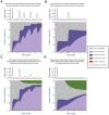
Fig. 4. Time series of the fraction of the population with severe primary or secondary cases (top) and area plots of the fraction of the population comprising each immune (S_P, R, S_S, V) or infection (I_P, I_S) class (bottom) over a 5-year time period under four different future scenarios.

In all plots, the relative transmissibility of secondary infections (α) is taken to be 1, the fraction of severe primary cases (x_sev,p) is assumed to be 0.14, a seasonal transmission rate derived from the climate of New York City with no lag is assumed, and a period of social distancing during which the force of infection is reduced to 60% of its original value during weeks 16 to 55 (i.e., the scenario described in Fig. 2B) is enforced. (A and B) Two scenarios in which no vaccination occurs: a more pessimistic natural immunity scenario, with ε = 0.7, 1/δ = 0.5 years, and 21% of secondary cases being severe (A) and a more optimistic natural immunity scenario, with ε = 0.5, 1/δ = 2 years, and 7% of secondary cases being severe (B). (C and D) Two scenarios in which vaccination is introduced at a weekly rate ν of 1% at t_vax of 1.5 years after the onset of the pandemic: with all the parameters in (A) along with vaccinal immunity lasting 1/δ_vax of 0.25 years (C) or with all the same parameters as in (B) along with vaccinal immunity lasting 1/δ_vax of 1 year (D).

Fig. 5. Effect of vaccine refusal on disease dynamics.

(A) Daily proportion of vaccine-adopting individuals from the partially and fully susceptible immune classes who must be immunized in order to achieve ℛ₀ < 1 as a function of the fraction of the population that refuses the vaccine (37) for different values of the duration of vaccinal immunity (1/δ_vax = 0.25 years, solid line; 1/δ_vax = 0.5 years, dashed line; 1/δ_vax = 1 year, dotted line) and different values of the susceptibility to secondary infection ε [ε = 0.5 (left) ε = 0.7 (middle) or ε = 1 right)]. (Top row) Homogeneous transmission between vaccine adopters and refusers (c₁₁ = c₁₂ = c₂₁ = c₂₂ = 1). (Middle row) Increased transmission associated with vaccine refusers (c₁₁ = 1, c₁₂ = 1.25, c₂₁ = 1.25, and c₂₂ = 1.5). (Bottom row) Decreased transmission associated with vaccine refusers (c₁₁ = 1, c₁₂ = 0.825, c₂₁ = 0.825, and c₂₂ = 0.75). (B) Maximum fraction of the population that can refuse vaccination for herd immunity to still be achieved as a function of the contact rate among vaccine refusers c₂₂ (37). In (A) and (B), the transmission rate is derived from the mean value of seasonal New York City–based weekly reproduction numbers (${\overline{R}}_0$ = 1.75) (37) (fig. S2C). (C) Time series of the fraction of the population with severe primary or secondary cases (top) and area plots of the fraction of the population comprising each immune (S_P, R, S_S, V) or infection (I_P, I_S) class (bottom) over a 5-year time period. The parameters in the left two series are identical to those in Fig. 4C, and the parameters in the right two series are identical to those in Fig. 4D. Additionally, the fraction of the population refusing vaccines is taken to be N₂ = 0.3. (Top row) Homogeneous mixing with c₁₁ = c₁₂ = c₂₁ = c₂₂ = 1. (Bottom row) Increased contacts among vaccine refusers and c₁₁ = 1, c₁₂ = 1.25, c₂₁ = 1.25, and c₂₂ = 1.5.

References

1. Laksono B. M., de Vries R. D., McQuaid S., Duprex W. P., de Swart R. L., Measles Virus Host Invasion and Pathogenesis. Viruses 8, 210 (2016). 10.3390/v8080210 - DOI - PMC - PubMed
1. Ellner P. D., Smallpox: Gone but not forgotten. Infection 26, 263–269 (1998). 10.1007/BF02962244 - DOI - PubMed
1. Dushoff J., Plotkin J. B., Levin S. A., Earn D. J. D., Dynamical resonance can account for seasonality of influenza epidemics. Proc. Natl. Acad. Sci. U.S.A. 101, 16915–16916 (2004). 10.1073/pnas.0407293101 - DOI - PMC - PubMed
1. Pitzer V. E., Viboud C., Alonso W. J., Wilcox T., Metcalf C. J., Steiner C. A., Haynes A. K., Grenfell B. T., Environmental drivers of the spatiotemporal dynamics of respiratory syncytial virus in the United States. PLOS Pathog. 11, e1004591 (2015). 10.1371/journal.ppat.1004591 - DOI - PMC - PubMed
1. Ferguson N., Anderson R., Gupta S., The effect of antibody-dependent enhancement on the transmission dynamics and persistence of multiple-strain pathogens. Proc. Natl. Acad. Sci. U.S.A. 96, 790–794 (1999). 10.1073/pnas.96.2.790 - DOI - PMC - PubMed
Publication types