Automatic contouring system for cervical cancer using convolutional neural networks

Abstract

Purpose: To develop a tool for the automatic contouring of clinical treatment volumes (CTVs) and normal tissues for radiotherapy treatment planning in cervical cancer patients.

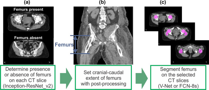
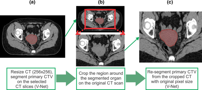
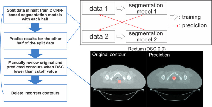
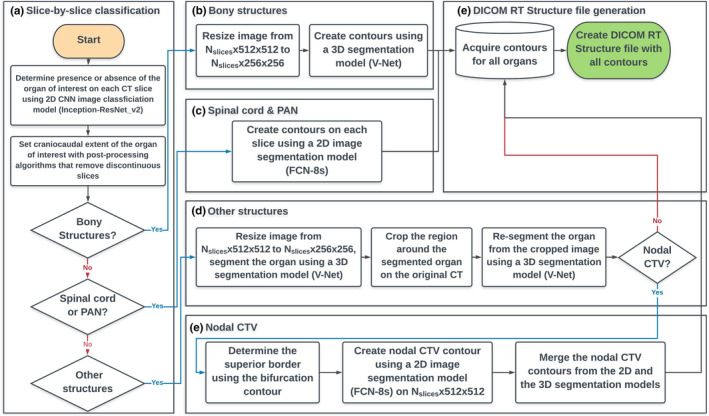
Methods: An auto-contouring tool based on convolutional neural networks (CNN) was developed to delineate three cervical CTVs and 11 normal structures (seven OARs, four bony structures) in cervical cancer treatment for use with the Radiation Planning Assistant, a web-based automatic plan generation system. A total of 2254 retrospective clinical computed tomography (CT) scans from a single cancer center and 210 CT scans from a segmentation challenge were used to train and validate the CNN-based auto-contouring tool. The accuracy of the tool was evaluated by calculating the Sørensen-dice similarity coefficient (DSC) and mean surface and Hausdorff distances between the automatically generated contours and physician-drawn contours on 140 internal CT scans. A radiation oncologist scored the automatically generated contours on 30 external CT scans from three South African hospitals.

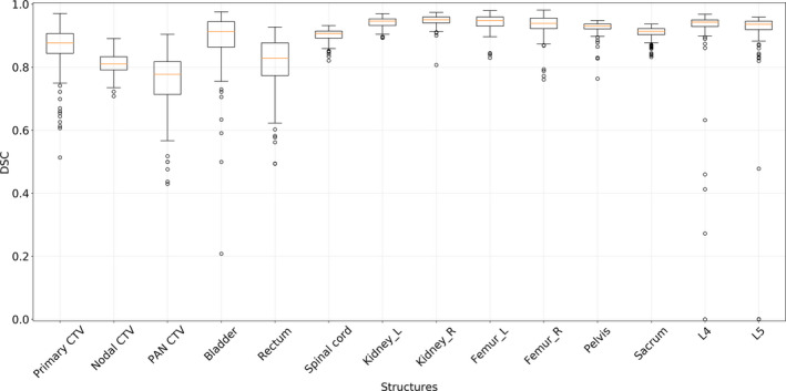
Results: The average DSC, mean surface distance, and Hausdorff distance of our CNN-based tool were 0.86/0.19 cm/2.02 cm for the primary CTV, 0.81/0.21 cm/2.09 cm for the nodal CTV, 0.76/0.27 cm/2.00 cm for the PAN CTV, 0.89/0.11 cm/1.07 cm for the bladder, 0.81/0.18 cm/1.66 cm for the rectum, 0.90/0.06 cm/0.65 cm for the spinal cord, 0.94/0.06 cm/0.60 cm for the left femur, 0.93/0.07 cm/0.66 cm for the right femur, 0.94/0.08 cm/0.76 cm for the left kidney, 0.95/0.07 cm/0.84 cm for the right kidney, 0.93/0.05 cm/1.06 cm for the pelvic bone, 0.91/0.07 cm/1.25 cm for the sacrum, 0.91/0.07 cm/0.53 cm for the L4 vertebral body, and 0.90/0.08 cm/0.68 cm for the L5 vertebral bodies. On average, 80% of the CTVs, 97% of the organ at risk, and 98% of the bony structure contours in the external test dataset were clinically acceptable based on physician review.

Conclusions: Our CNN-based auto-contouring tool performed well on both internal and external datasets and had a high rate of clinical acceptability.

Keywords: auto-contouring; cervical cancer; convolutional neural network; deep learning.

Fig. 1

Application of the convolutional neural network‐based classification and segmentation models to a computed tomography (CT) scan. (a) The presence or absence of the organ of interest (in this case, femurs) was evaluated on each CT slice, (b) the cranial‐caudal extent of the organ of interest was determined with postprocessing, and (c) the slices that were classified to contain the organ of interest were used in the segmentation model to generate contours. [Color figure can be viewed at wileyonlinelibrary.com]

Fig. 2

Segmentation using cropped three‐dimensional images for better accuracy. (a) Resize the computed tomography (CT) from 512 × 512 to 256 × 256 pixels and then segment the organ of interest and find the center of mass, (b) crop the region around the segmented organ on the original 512 × 512 CT scan, and (c) resegment the organ of interest on the cropped image. [Color figure can be viewed at wileyonlinelibrary.com]

Fig. 3

Flowchart of the semi‐automated data curation method to identify incorrect clinical contours. Data were randomly split into two groups, and two auto‐segmentation models were trained with each dataset. Then, each segmentation model was applied to the other group of data to create contours. If the Sørensen‐Dice similarity coefficient was lower than the threshold value, the original contour was manually reviewed and deleted if incorrect. [Color figure can be viewed at wileyonlinelibrary.com]

Fig. 4

Overall flowchart of the developed auto‐contouring system for cervical cancer. (a) The slice by slice classification was conducted to identify computed tomography (CT) slices that contain a target structure, and the process is visually demonstrated in Fig. 1. (b) Bony structures were contoured as described in Section 2.B. (c) Spinal cord and PAN clinical treatment volume (CTV) were contoured with the 2D FCN‐8s segmentation architecture. (d) Other structures (the organs‐at‐risk and the primary and the nodal CTVs) were contoured as demonstrated in Fig. 2. (e) Extra steps were required for the nodal CTV contours as described in Section 2.C.2. [Color figure can be viewed at wileyonlinelibrary.com]

Fig. 5

The distributions of Sørensen‐Dice similarity coefficients between the ground truth and the automatically generated contours of 14 structures. [Color figure can be viewed at wileyonlinelibrary.com]

Fig. 6

The outlier contours from the internal test dataset. The ground truth contours (green) and outliers (red) are given for (a) primary clinical treatment volume (CTV) (Sørensen‐Dice similarity coefficient [DSC] = 0.43), (b) bladder (DSC = 0.21), (c) L4 and L5 vertebral bodies (DSC = 0.0 each), and (d) PAN CTV (DSC = 0.43). [Color figure can be viewed at wileyonlinelibrary.com]

Fig. 7

Examples of automatically generated contours (red) vs ground truth (green) from physician’s manual review of contours for the primary clinical treatment volume, bladder, and rectum. [Color figure can be viewed at wileyonlinelibrary.com]

Fig. 8

The aortic bifurcation is clearly defined in the red box in (a), whereas the aortic bifurcation is barely identifiable in the red box in (b). The adjustment of the window level did not improve the visual inspection. [Color figure can be viewed at wileyonlinelibrary.com]

References

-
- Vorwerk H, Zink K, Schiller R, et al. Protection of quality and innovation in radiation oncology: the prospective multicenter trial the German Society of Radiation Oncology (DEGRO‐QUIRO study). Strahlentherapie und Onkol. 2014;190:433–443. - PubMed
- Andrianarison VA, Laouiti M, Fargier‐Bochaton O, et al. Contouring workload in adjuvant breast cancer radiotherapy. Cancer Radiother. 2018;22:747–753. - PubMed
- Yang J, Zhang Y, Zhang L, Dong L. Automatic segmentation of parotids from CT scans using multiple atlases Medical Image Analysis for the Clinic: A Grand Challenge. 2010:223–230.
MeSH terms
Grants and funding
LinkOut - more resources
Full Text Sources
Other Literature Sources