Whole-Brain Image Analysis and Anatomical Atlas 3D Generation Using MagellanMapper

Abstract

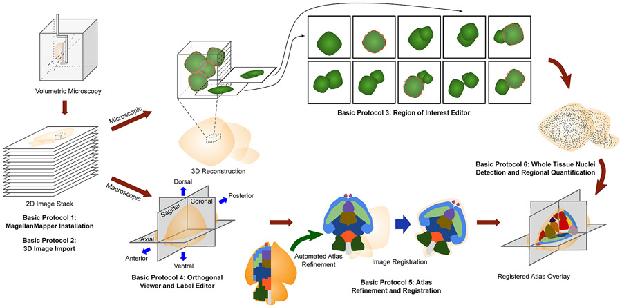
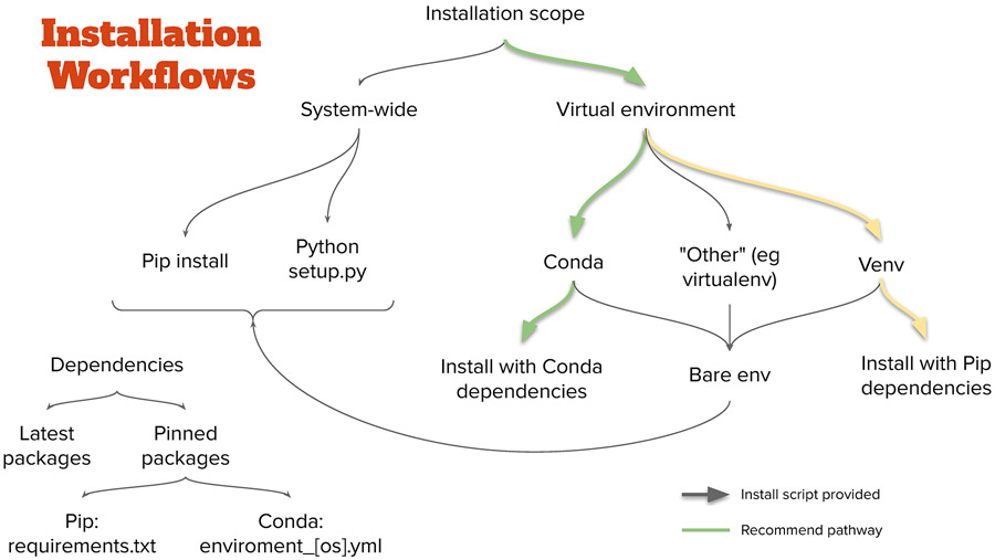
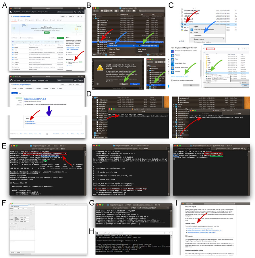
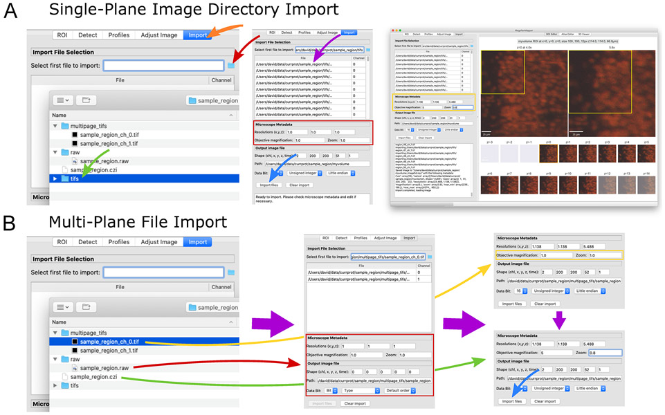
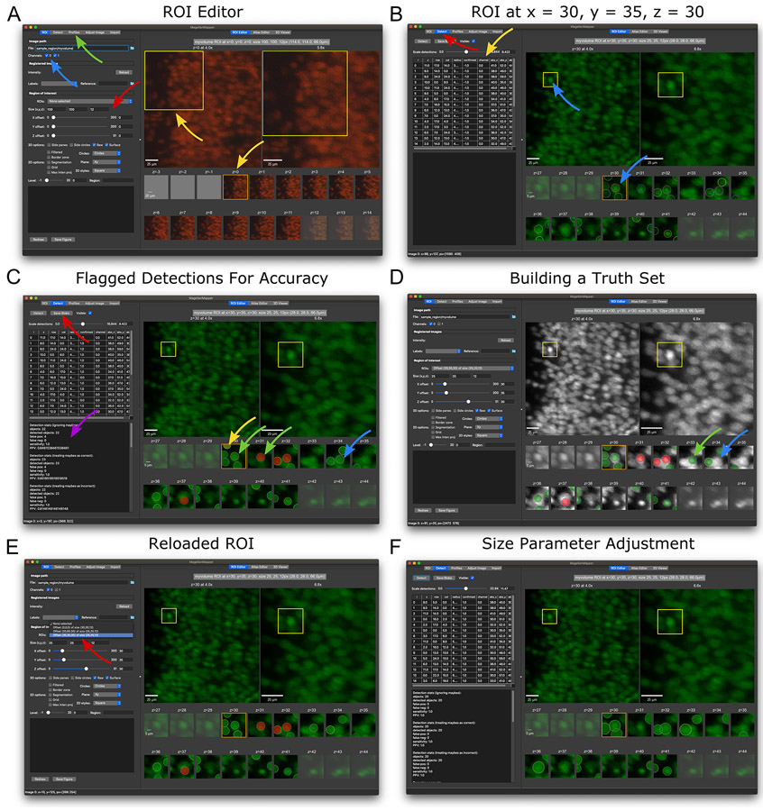
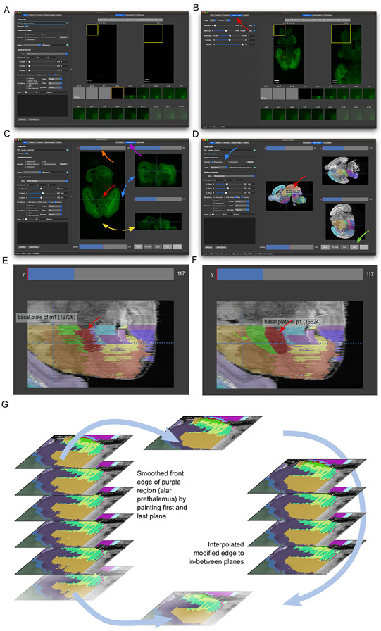
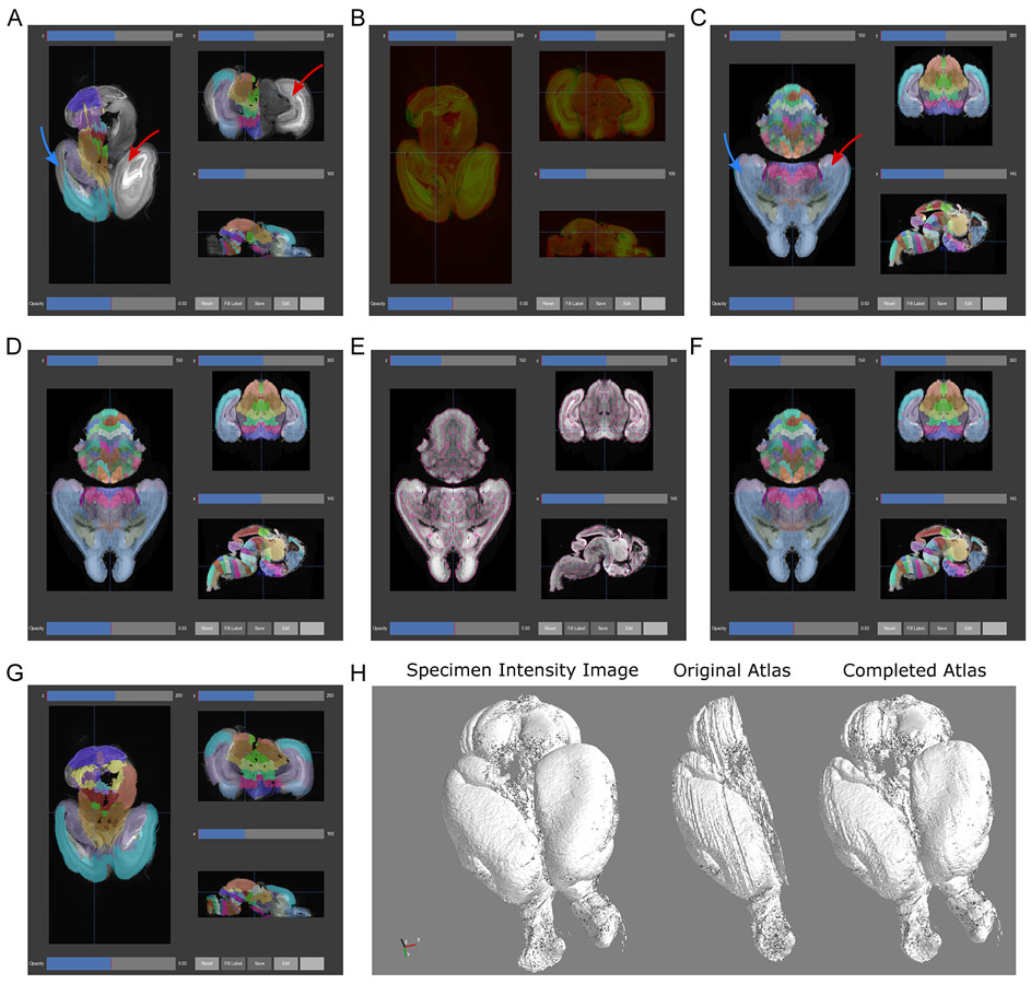
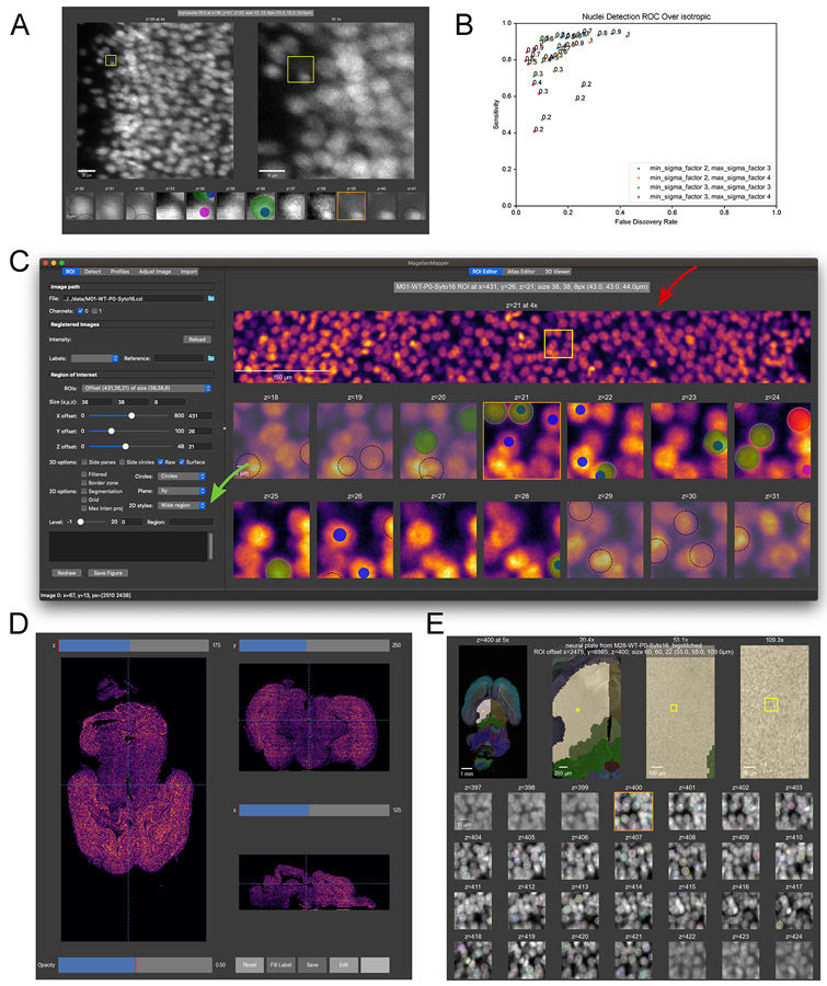
MagellanMapper is a software suite designed for visual inspection and end-to-end automated processing of large-volume, 3D brain imaging datasets in a memory-efficient manner. The rapidly growing number of large-volume, high-resolution datasets necessitates visualization of raw data at both macro- and microscopic levels to assess the quality of data, as well as automated processing to quantify data in an unbiased manner for comparison across a large number of samples. To facilitate these analyses, MagellanMapper provides both a graphical user interface for manual inspection and a command-line interface for automated image processing. At the macroscopic level, the graphical interface allows researchers to view full volumetric images simultaneously in each dimension and to annotate anatomical label placements. At the microscopic level, researchers can inspect regions of interest at high resolution to build ground truth data of cellular locations such as nuclei positions. Using the command-line interface, researchers can automate cell detection across volumetric images, refine anatomical atlas labels to fit underlying histology, register these atlases to sample images, and perform statistical analyses by anatomical region. MagellanMapper leverages established open-source computer vision libraries and is itself open source and freely available for download and extension. © 2020 Wiley Periodicals LLC. Basic Protocol 1: MagellanMapper installation Alternate Protocol: Alternative methods for MagellanMapper installation Basic Protocol 2: Import image files into MagellanMapper Basic Protocol 3: Region of interest visualization and annotation Basic Protocol 4: Explore an atlas along all three dimensions and register to a sample brain Basic Protocol 5: Automated 3D anatomical atlas construction Basic Protocol 6: Whole-tissue cell detection and quantification by anatomical label Support Protocol: Import a tiled microscopy image in proprietary format into MagellanMapper.

Keywords: 3D atlas; graphical interface; image processing; microscopy images; tissue clearing.

Figure 1.

Overview of MagellanMapper features and workflow for image processing of volumetric imaging. Volumetric microscopy sources include serial two-photon tomography (STPT), lightsheet imaging of tissue cleared specimen, or in vivo imaging such as MRI typically produce stacks of inherently aligned serial 2D sections that can be merged into a 3D reconstruction. MagellanMapper facilitates visualization and annotation of images at the microscopic and macroscopic scale. Basic Protocol 1 describes installation of MagellanMapper, while Basic Protocol 2 provides instruction on importing a variety of image formats into MagellanMapper. In Basic Protocol 3, we describe the Region of Interest (ROI) Editor for viewing small windows of high resolution data in a 3D context through each plane in the ROI. Automated 3D nuclei detection places circles indicating object location, and annotation tools in the editor allow repositioning, modifying, and adding or subtracting circles. Basic Protocol 4 describes the Atlas Editor used to view images at a macroscopic scale by providing simultaneous views of planes along each axis and painting tools to markup structures. Basic Protocol 5 gives instruction on atlas 3D reconstruction and registration, including tools that can take partially labeled, 2D-derived atlases and automatically complete and generate 3D atlases based on the underlying anatomical signal. This registration provides the anatomical demarcations necessary for Basic Protocol 6, which describes whole tissue 3D image processing of nuclei for quantification by anatomical region.

Figure 2.

Installation pathways. As with many Python applications, MagellanMapper can be installed through several pathways. The recommended pathway is through Conda, which handles all required dependencies and keeps them separate from any other installed Python packages in a virtual environment. For those who prefer a more “pure Python” approach, Venv will also keep packages separate in an environment while installing dependencies through Pip. Installation scripts are provided to simplify the Conda pathway. Various other pathways are also available. Typically, the latest dependencies are installed, but specifications that pin each dependency version are available for reproducibility.

Figure 3.

Installation screenshots. (A) The MagellanMapper software GitHub website hosts the software source code and serves as a portal for community involvement including posting issues for support and additional instructions on using the software. The “releases” link (top, red arrow) links to the MagellanMapper version releases page. At the bottom of each release, the source code can be downloaded as a single compressed file (bottom, red arrow). (B) After extracting the compressed file, the Conda setup script can be launched from the bin folder. On Mac (top), the file can be launched by right-clicking the file (red arrow), choosing “Open with…” (blue arrow), and selecting the Terminal app (green arrow). This process will allow the security prompt to be accepted (bottom left, green arrow). After installation, double-clicking the MagellanMapper file (bottom right, green arrow) will launch the software. (C) On Windows, the Python run script can be launched by associating Python files with the Python application installed with Conda. Right-clicking the run script (top, red arrow) and choosing “Open with…” (blue arrow) allows the user to look for an app to open the file (bottom left, green arrow). In the Miniconda folder (bottom right, red box), the Python executable can be selected (green arrow). (D) Alternatively, the Conda setup script can be dragged into a terminal will copy that path into the command-line (left). Pressing Enter will initiate the script to install MagellanMapper. After installation, dragging the run script into the terminal and pressing Enter will launch MagellanMapper as shown in part F (right). (E) Installation and running MagellanMapper can also be initiated fully in a terminal. After typing “cd ” (space included), the folder can be typed in directly, or dragged into the terminal similarly as before (left, red rectangle). Pressing Enter enters that folder. Typing the path to the install script (blue rectangle, here shown for Mac and Linux) and pressing Enter starts the installation process. In this case, Conda is not found and thus downloaded and installed after confirmation from the user (green rectangle). Since Conda was just installed, a new terminal will need to be opened after installation completes (middle, red rectangle). After opening a new terminal, the Conda activation command will start the newly created MagellanMapper environment (left, red rectangle). The “(mag)” at the start of the line indicates that the environment has been successfully activated (blue rectangle). The MagellanMapper launch command can now be entered (green rectangle) to (F) open MagellanMapper. (G) If Conda is already installed, the MagellanMapper install script skips Conda installation and proceeds directly to creating a new environment. (H) Equivalent install script for Windows systems. (KI) The website home page also hosts sample 3D data for use in these Protocols.

Figure 4.

Import image files into a Numpy volumetric format. (A) The “Import” panel (left, orange arrow) displays selectors for choosing a file (red arrow), such as a directory of images (green arrow). The files are loaded into the table (middle, purple arrow) with channel determined based on the filename. Microscopy metadata can be entered (red box) and pressing the “Import files” button loads (blue arrow) each image file into a separate plane of a single volumetric image file (right). (B) Several types of multi-plane images can be loaded (left). Raw image formats typically contain no metadata (red arrow), and all metadata should be entered manually. For multi-plane, multichannel TIFF files, selecting the first file (yellow arrow) will cause related files to be loaded into the table (middle). In the metadata area (middle, red box), image parameters will be loaded based on available metadata embedded in the file. In this case, partial metadata is loaded, and the rest needs to be entered manually (right, yellow box). Some proprietary formats (green arrow) contain all channels and metadata in a single file, allowing immediate import (right, blue arrow).

Figure 5.

Detecting and annotating nuclei in the ROI Editor. (A) The main graphical interface for MagellanMapper shows options for defining and visualizing a region of interest (ROI) on the left, with the ROI displayed on the right. The ROI settings (red arrow) can be entered in the size boxes and offset sliders. Below the ROI selection controls are various 2D and 3D viewing options, and further down are figure redraw and save controls. Channels can be toggled (blue arrow), and profiles changed in the Profiles tab (green arrow). In the right panel, the top row shows overview plots starting with the original image on the left and progressively zooming into the ROI highlighted by a yellow box with each successive plot (top yellow arrow), with. As a volumetric image, the full image contains multiple z-planes. The z-planes within the ROI are shown as smaller plots in the bottom rows, labeled by the corresponding absolute z-plane number (starting with z = 0). Scrolling the mouse or pressing arrow keys will scroll the original image’s z-plane and shift the orange box to the corresponding ROI z-plane (bottom yellow arrow). (B) A new ROI with different offset and size parameters as shown in the left panel settings. Whereas the previous view overlaid all channels, only the first channel was selected here. Selecting the “Detect” tab (red arrow) and pressing the “Detect” button will perform 3D blob detection to identify objects such as nuclei. The detected locations appear as circles in the ROI plots, with each circle positioned at the detected center of the given blob. Notice how the bright nucleus in the middle of the yellow box corresponds to a detection shown in the z = 30 ROI plot (blue arrows). The table shows the coordinates of each circle (yellow arrow). (C) Annotating detections based on accuracy. These circles can be repositioned, added, deleted, or flagged to assess detection accuracy and annotate ground truth sets to train the detector. Clicking on circles changes their color to flag them as correct (green circle, green arrow) or incorrect (red circle, red arrow). A yellow flag (yellow circle, yellow arrow) can be used for ambiguous detections or nuclei. Missing detections can be added by Ctrl-clicking on the desired location. After saving annotations (red arrow), detection statistics are shown in the feedback panel (purple arrow). (D) An example of further annotating the ROI to build ground truth by shifting, resizing, and copying/cutting/pasting circles. An alternate colormap assists with contrast for more precise annotation. Note the circle cut from z = 33 (blue arrows in parts C and D) and pasted into the next plane (z = 34, green arrow) to match the center of the nucleus along the z-axis. (E) After saving the ROI, the ROI appears in a dropdown box (red arrow), which can be selected to restore the ROI after shifting to a different ROI or re-opening MagellanMapper. (F) Cell detection parameter adjustment. Changing the minimum and maximum detection sizes can impact detection accuracy. In this case, the detected sizes of each nuclei are somewhat large, but the number of duplicate detections of the same nuclei decreases.

Figure 6.

Annotating labels in the Atlas Editor. (A) Opening the sample brain in MagellanMapper initially shows the bottom z-plane in the ROI Editor. (B) Scrolling a mouse moves the overview plots’ z-plane, while clicking on the plot moves the ROI offset controls to that position and shows a preview of the ROI (dashed box). Opening the image adjustment tab (red arrow) allows brightness and contrast control. (C) Opening the Atlas Editor tab (purple arrow) shows a simultaneous orthogonal viewer of the sample brain. Scrolling through the horizontal (axial, z, or xy-plane) plane or clicking/dragging its slider (orange arrow) moves through these planes. Clicking within the plane moves the crosshairs (red arrow) and shifts the coronal (y, or xz-plane; blue arrows) and sagittal (x, or yz-plane; yellow arrows) views to the planes corresponding to these crosshair lines. (D) The Allen Developing Mouse Brain E18.5 atlas is shown with the specified labels (blue arrow) overlaid on the microscopy intensity image. Each distinct label color corresponds to a separate label in the Allen ontology. Hovering over a given label identifies its name and Allen ID (red arrow). The tools at the bottom of the editor (green arrow) allow label display adjustment as well as edit controls for painting labels in each 2D plane. (E) Example y-plane before editing, showing jagged label edges. The white bordered ellipse shows the paint brush (red arrow), whose size can be adjusted using the bracket keys. (F) The red (red arrow) and green (green arrow) regions have been smoothed by simply dragging the brush along the label borders. (G) Example edge interpolation to smooth a label edge. Painting successive planes in 2D can lead to jagged edges when viewed in the third dimension. To paint smoothly in 3D, the label fill tool (green arrow section in part D) interpolates label edits between two separate planes. The alar prethalamus (purple label) shows jagged artifacts in each plane, including irregularity between each plane (left). The anterior edge of the label has been edited in the top and bottom planes to smooth the jaggedness (middle), without touching the middle four planes. Applying the edge interpolation applies the edits from the two manually edited planes smoothly along these unedited planes. After edits, the image can be saved (green arrow section in part D).

Figure 7.

Atlas registration and automated refinement. (A) Registration of the original Allen Developing Mouse Brain Atlas E18.5 atlas to the sample P0 mouse brain. After registration, the existing labels approximate the position, orientation, size, and shape of the corresponding parts of the sample brain. Note the missing labels in one entire hemisphere (red arrow) and the lateral planes of the labeled hemisphere (blue arrow). (B) Overlay of the sample brain (green) and registered atlas (red) intensity images as a qualitative assessment of registration. Misalignments can be optimized by adjusting settings in the software’s atlas profiles. (C) The automated 3D atlas generation pipeline performs extension of lateral labels into the unlabeled areas (blue arrow) by iteratively growing the existing labels to fit the anatomical contours (part F). After extending the lateral labels, the unlabeled hemisphere is replaced by mirroring the labeled hemisphere (red arrow), resulting in a fully labeled atlas in 3D. (D) Label smoothing removed many of the jagged artifacts most visible in the axial and coronal planes. (E) To further smooth and refine labels, edge detection (pink lines) of gross anatomical boundaries (high grayscale contrast) in the microscopy intensity image provides a 3D guide for aligning label edges. (F) Starting with the atlas from part C, each label is eroded to its core and regrown by a watershed algorithm guided by the anatomical map from part E, followed by smoothing as in part D to remove small artifacts from the watershed. (G) The same registration as performed in part A is performed but with the generated 3D atlas labels. (H) The 3D Viewer provides a macroscopic view of the specimen through 3D surface rendering of the sample brain (left). Surface rendering of the registered labels (center) before and (right) after 3D atlas generation demonstrate label completion and smoothing.

Figure 8.

Whole brain nuclei detection and assignment to anatomical labels. (A) Automated verification within the depicted sub-ROI shows truth blobs as small, opaque dots and detections as larger, translucent circles. Blue dots are correctly detected truth blobs, while purple dots are misses. Green circles are correct detections, and red circles are false. Correct detections and corresponding truth blobs may be separated by up to a few z-planes if the detector correctly identified a nucleus but slightly off its center in the z-axis. The interface allows inspection to determine where the detector may have worked or failed to guide further optimization. (B) A receiver operating characteristic (ROC) curve from a Grid Search test of several combinations of detection setting parameters with more ROIs of larger size. The minimum and maximum object size parameters and an isotropic scaling factor were varied, with the false discovery rate (FDR, x-axis) and sensitivity (y-axis) shown for each combination. The point labels show the isotropic factor (1 = isotropic, 0.5 = z-scale is half that of x and y), and the color and point symbol correspond to the legend values denoting min/max size parameters. (C) Example of automated verifications in one of these larger ROIs. A sub-image (red arrow) was extracted from the original whole-brain image and 10 ROIs annotated as ground truth, and a wide layout was selected (green arrow). (D) Density heat map of nuclei detected across a full-resolution sample brain using the pipelines script. (E) High resolution serial 2D plots from the ROI Editor show the individual detected nuclei. The ROI coordinates were found by specifying a region ID (below the green arrow in part C), Allen ID 16382 (the alar thalamus, showing the left side), which positioned the ROI to the center of this label. Overview plots show the ROI in context with anatomical labels overlaid and the left alar thalamus highlighted in light gold.

References

1. Allen Institute for Brain Science. (n.d.). API - Allen Developing Mouse Brain Atlas. Retrieved July 3, 2019, from http://help.brain-map.org/display/devmouse/API
1. Cai R, Pan C, Ghasemigharagoz A, Todorov MI, Förstera B, Zhao S, … Ertürk A (2019). Panoptic imaging of transparent mice reveals whole-body neuronal projections and skull–meninges connections. Nature Neuroscience, 22(2), 317 10.1038/s41593-018-0301-3 - DOI - PMC - PubMed
1. Fürth D, Vaissière T, Tzortzi O, Xuan Y, Märtin A, Lazaridis I, … Meletis K (2018). An interactive framework for whole-brain maps at cellular resolution. Nature Neuroscience, 21(1), 139 10.1038/s41593-017-0027-7 - DOI - PMC - PubMed
1. Hörl D, Rusak FR, Preusser F, Tillberg P, Randel N, Chhetri RK, … Preibisch S (2019). BigStitcher: Reconstructing high-resolution image datasets of cleared and expanded samples. Nature Methods, 16(9), 870–874. 10.1038/s41592-019-0501-0 - DOI - PubMed
1. Hunter JD (2007). Matplotlib: A 2D Graphics Environment. Computing in Science Engineering, 9(3), 90–95. 10.1109/MCSE.2007.55 - DOI
Publication types