

Deep learning-based reduced order models in cardiac electrophysiology
- PMID: 33002014
- PMCID: PMC7529269
- DOI: 10.1371/journal.pone.0239416
Deep learning-based reduced order models in cardiac electrophysiology
Abstract
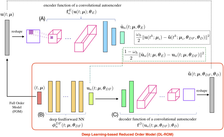
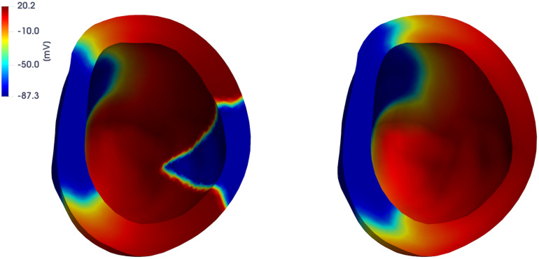
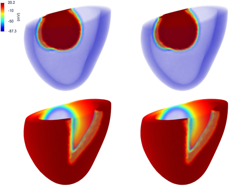
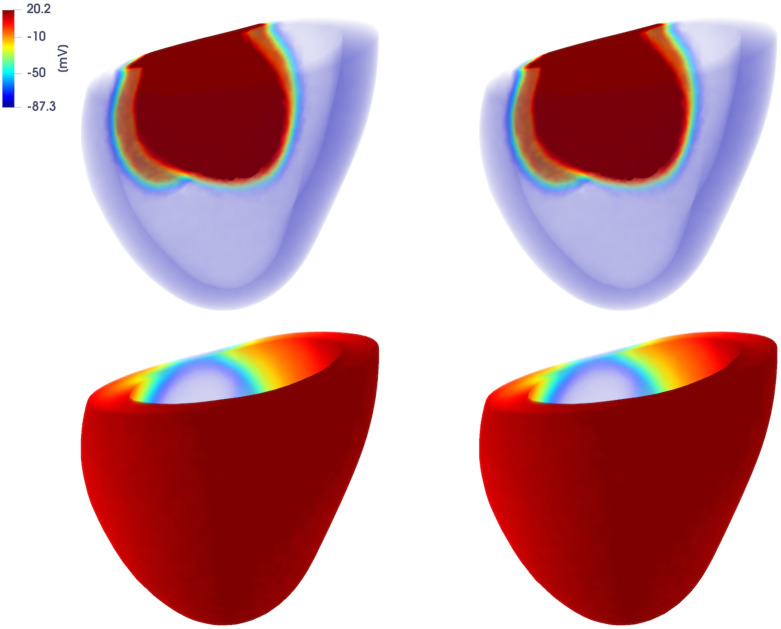
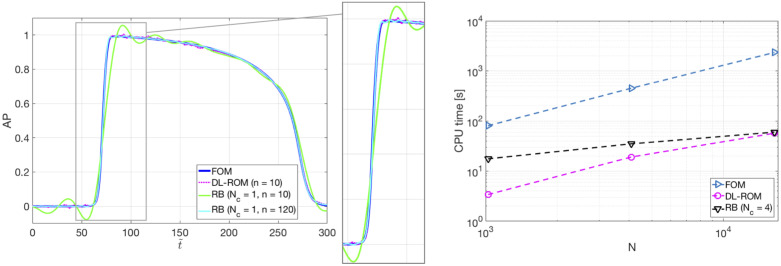
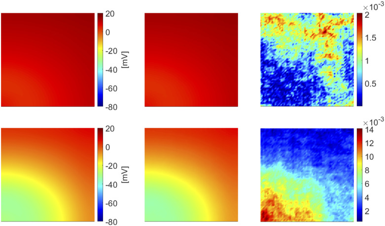
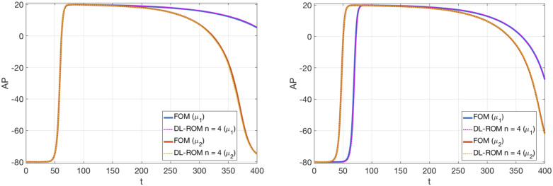
Predicting the electrical behavior of the heart, from the cellular scale to the tissue level, relies on the numerical approximation of coupled nonlinear dynamical systems. These systems describe the cardiac action potential, that is the polarization/depolarization cycle occurring at every heart beat that models the time evolution of the electrical potential across the cell membrane, as well as a set of ionic variables. Multiple solutions of these systems, corresponding to different model inputs, are required to evaluate outputs of clinical interest, such as activation maps and action potential duration. More importantly, these models feature coherent structures that propagate over time, such as wavefronts. These systems can hardly be reduced to lower dimensional problems by conventional reduced order models (ROMs) such as, e.g., the reduced basis method. This is primarily due to the low regularity of the solution manifold (with respect to the problem parameters), as well as to the nonlinear nature of the input-output maps that we intend to reconstruct numerically. To overcome this difficulty, in this paper we propose a new, nonlinear approach relying on deep learning (DL) algorithms-such as deep feedforward neural networks and convolutional autoencoders-to obtain accurate and efficient ROMs, whose dimensionality matches the number of system parameters. We show that the proposed DL-ROM framework can efficiently provide solutions to parametrized electrophysiology problems, thus enabling multi-scenario analysis in pathological cases. We investigate four challenging test cases in cardiac electrophysiology, thus demonstrating that DL-ROM outperforms classical projection-based ROMs.
Conflict of interest statement
The authors have declared that no competing interests exist.
Figures
Similar articles
-
POD-Enhanced Deep Learning-Based Reduced Order Models for the Real-Time Simulation of Cardiac Electrophysiology in the Left Atrium.Front Physiol. 2021 Sep 22;12:679076. doi: 10.3389/fphys.2021.679076. eCollection 2021. Front Physiol. 2021. PMID: 34630131 Free PMC article.
-
Efficient approximation of cardiac mechanics through reduced-order modeling with deep learning-based operator approximation.Int J Numer Method Biomed Eng. 2024 Jan;40(1):e3783. doi: 10.1002/cnm.3783. Epub 2023 Nov 3. Int J Numer Method Biomed Eng. 2024. PMID: 37921217
-
Enabling forward uncertainty quantification and sensitivity analysis in cardiac electrophysiology by reduced order modeling and machine learning.Int J Numer Method Biomed Eng. 2021 Jun;37(6):e3450. doi: 10.1002/cnm.3450. Epub 2021 May 7. Int J Numer Method Biomed Eng. 2021. PMID: 33599106 Free PMC article.
-
Uncertainty quantification of fast sodium current steady-state inactivation for multi-scale models of cardiac electrophysiology.Prog Biophys Mol Biol. 2015 Jan;117(1):4-18. doi: 10.1016/j.pbiomolbio.2015.01.008. Epub 2015 Feb 7. Prog Biophys Mol Biol. 2015. PMID: 25661325 Free PMC article. Review.
-
Nonlinear dynamics in cardiac conduction.Math Biosci. 1988;90:19-48. doi: 10.1016/0025-5564(88)90056-9. Math Biosci. 1988. PMID: 11539069 Review.
Cited by
-
Whole-heart ventricular arrhythmia modeling moving forward: Mechanistic insights and translational applications.Biophys Rev (Melville). 2021 Sep;2(3):031304. doi: 10.1063/5.0058050. Epub 2021 Sep 28. Biophys Rev (Melville). 2021. PMID: 36281224 Free PMC article.
-
POD-Enhanced Deep Learning-Based Reduced Order Models for the Real-Time Simulation of Cardiac Electrophysiology in the Left Atrium.Front Physiol. 2021 Sep 22;12:679076. doi: 10.3389/fphys.2021.679076. eCollection 2021. Front Physiol. 2021. PMID: 34630131 Free PMC article.
-
Fast and accurate prediction of drug induced proarrhythmic risk with sex specific cardiac emulators.NPJ Digit Med. 2024 Dec 26;7(1):380. doi: 10.1038/s41746-024-01370-8. NPJ Digit Med. 2024. PMID: 39725693 Free PMC article.
-
A Review of Healthy and Fibrotic Myocardium Microstructure Modeling and Corresponding Intracardiac Electrograms.Front Physiol. 2022 May 10;13:908069. doi: 10.3389/fphys.2022.908069. eCollection 2022. Front Physiol. 2022. PMID: 35620600 Free PMC article. Review.
-
Data integration for the numerical simulation of cardiac electrophysiology.Pacing Clin Electrophysiol. 2021 Apr;44(4):726-736. doi: 10.1111/pace.14198. Epub 2021 Mar 8. Pacing Clin Electrophysiol. 2021. PMID: 33594761 Free PMC article. Review.
References
-
- Quarteroni A, Manzoni A, Vergara C. The cardiovascular system: Mathematical modeling, numerical algorithms, clinical applications. Acta Numerica. 2017;26:365–590. 10.1017/S0962492917000046 - DOI
-
- Quarteroni A, Dedè L, Manzoni A, Vergara C. Mathematical modelling of the human cardiovascular system: Data, numerical approximation, clinical applications Cambridge Monographs on Applied and Computational Mathematics. Cambridge University Press; 2019.
-
- Colli Franzone P, Pavarino LF, Scacchi S. Mathematical cardiac electrophysiology vol. 13 of MS&A. Springer; 2014.
-
- Sundnes J, Lines GT, Cai X, Nielsen BF, Mardal KA, Tveito A. Computing the electrical activity in the heart. vol. 1 Springer Science & Business Media; 2007.
-
- Colli Franzone P, Pavarino LF. A parallel solver for reaction–diffusion systems in computational electrocardiology. Mathematical Models and Methods in Applied Sciences. 2004;14(06):883–911. 10.1142/S0218202504003489 - DOI
Publication types
MeSH terms
LinkOut - more resources
Full Text Sources
