Robust parallel decision-making in neural circuits with nonlinear inhibition

Abstract

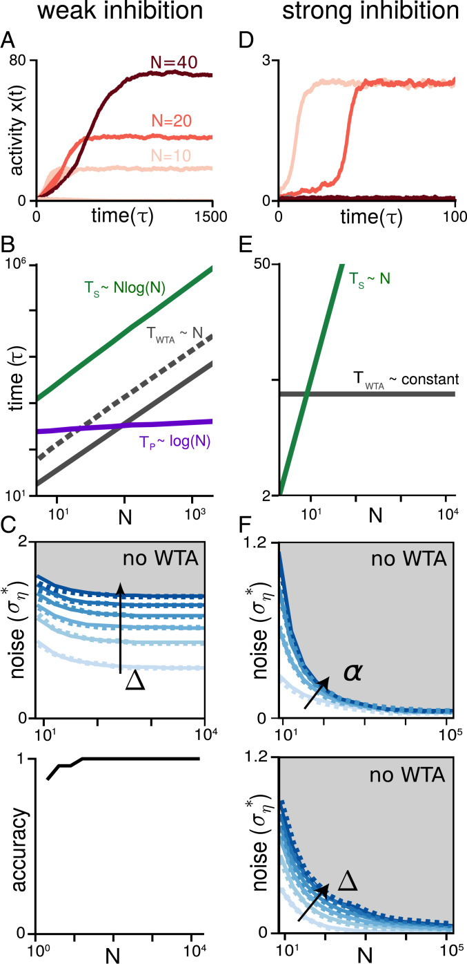
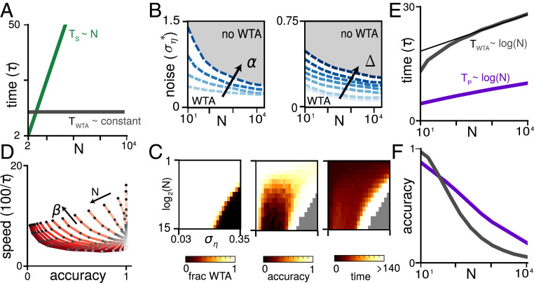
An elemental computation in the brain is to identify the best in a set of options and report its value. It is required for inference, decision-making, optimization, action selection, consensus, and foraging. Neural computing is considered powerful because of its parallelism; however, it is unclear whether neurons can perform this max-finding operation in a way that improves upon the prohibitively slow optimal serial max-finding computation (which takes [Formula: see text] time for N noisy candidate options) by a factor of N, the benchmark for parallel computation. Biologically plausible architectures for this task are winner-take-all (WTA) networks, where individual neurons inhibit each other so only those with the largest input remain active. We show that conventional WTA networks fail the parallelism benchmark and, worse, in the presence of noise, altogether fail to produce a winner when N is large. We introduce the nWTA network, in which neurons are equipped with a second nonlinearity that prevents weakly active neurons from contributing inhibition. Without parameter fine-tuning or rescaling as N varies, the nWTA network achieves the parallelism benchmark. The network reproduces experimentally observed phenomena like Hick's law without needing an additional readout stage or adaptive N-dependent thresholds. Our work bridges scales by linking cellular nonlinearities to circuit-level decision-making, establishes that distributed computation saturating the parallelism benchmark is possible in networks of noisy, finite-memory neurons, and shows that Hick's law may be a symptom of near-optimal parallel decision-making with noisy input.

Keywords: neural circuits; noisy computation; optimal decision-making; speed–accuracy trade-off.

Fig. 1.

Parallelism benchmarks and setup of the WTA circuit. (A) Schematic illustration of how $\log \left(N\right)$ integration time is sufficient to maintain fixed accuracy (here measured as number of correct trials over total number of trials). Thin lines denote sample time series from different trials for each option ($N$ options are in different colors; here $N=4$). Thick curves denote sample histograms (distributions) after integrating for time $T$. The tails of the distribution shrink exponentially (shown by gray shading). Thus, integrating for time $\log \left(N\right)$ means a per-option error probability of $\sim 1/N$, so that the total error probability, given by $N$ times the per-option error probability, is fixed. (B) The $\log \left(N\right)$ integration time is necessary to maintain fixed accuracy when estimating the means of noisy time series with Gaussian fluctuations. Plot shows the integration time to fixed accuracy (dashed and solid lines, $80\%$ and $99\%$ accuracy, respectively) in (nonneural) simulations with Gaussian input fluctuations. Thin black lines are logarithmic fits. (C) WTA network architectures. (Top) The time series $b_i$ serve as input to $N=4$ neurons (or pools of neurons), ordered by the size of their constant mean (with gap $\mathrm{\Delta }\equiv b_1-b_2$ between the top two inputs). Each neuron pool inhibits all others and excites itself. (Bottom) Mathematically equivalent network with a global inhibitory neuron pool: All neuron pools excite the inhibitory neuron pool, which inhibits them. This requires only $\sim N$ synapses, compared to $N^2$ for the mutual inhibition circuit (Top). (D) Neural firing rates and synaptic activations (coloring as in C). Convergence time $T_{\text{WTA}}$ is the time taken for the firing rate of the winner neuron pool to reach a fraction $c$ (usually chosen as 0.8; see Methods) of its expected asymptotic activity $x^{\infty }$ (black line). Dashed line denotes threshold for a neuron pool to contribute inhibition in the nonlinear inhibition model (nWTA; see Methods).

Fig. 2.

Conventional WTA networks fail the parallelism benchmark. (A–C) Results for weak inhibition. (A) Activity dynamics of the most active neuron (pool) for networks of size $N=\mathrm{10,20,40}$ (light to dark red), respectively, with noisy input; $\alpha =0.6$, $\beta =1$, $\mathrm{\Delta }=0.1$, ${\sigma }_{\eta }=0.35$, ${\tau }_{\eta }=0.05\tau$. The asymptotic activity level grows with $N$. (B) WTA simulation results on decision time without (solid gray) and with (dashed gray) noise. Also shown are noisy serial strategy (green) and noisy parallelism benchmark (purple). Note that benchmarks are shown up to an overall constant. Error bars are smaller than the line width. Deterministic serial strategy (i.e., $O\left(N\right)$) is not shown, for simplicity. (C) (Top) Critical noise amplitude versus $N$: WTA dynamics exists below a given curve and fails above it (dashed curve, numerical simulation; solid curve, analytical). Darker curves correspond to a larger gap between the top two inputs ($\mathrm{\Delta }=\left\{0.01,0.06,\dots ,0.26\right\}$, $\alpha =1-1/2N$, ${\tau }_{\eta }=0.005\tau$). (Bottom) Average accuracy, that is, fraction of correct trials, as a function of $N$ (simulations averaged over 150 trials). (D–F) Results for strong inhibition. (D) As in A but for strong inhibition. WTA breaks down rapidly (note absence of WTA for $N$ = 40, dark curve). (E) WTA decision time in the absence of noise (gray) along with the deterministic serial strategy (green). (F) As in C, showing critical noise amplitude versus $N$. Darker curves denote stronger self-excitation (Top; $\alpha =\left\{0.1,0.6,0.9,1.1\right\}$; $\mathrm{\Delta }=0.1$) or a widening gap (Bottom; $\mathrm{\Delta }=\left\{0.01,0.06,\dots ,0.26\right\}$; $\alpha =0.6$). $\beta =1$, in all curves.

Fig. 3.

The nWTA is robust to noise and achieves the parallelism benchmark. (A) The nWTA decision time without noise (gray) and the deterministic serial strategy (green). (B) Critical noise amplitude ${\sigma }_{\eta }*$ as a function of $N$ for varying $\alpha =\left\{0.5,0.7,0.9,1.1\right\}$, $\mathrm{\Delta }=0.075$ (Left) and $\mathrm{\Delta }=\left\{\mathrm{0,0.0125},0.025,0.05,0.075,0.1,0.15\right\}$, $\alpha =0.5$, $\beta =0.51$ (Right). Below each curve, WTA behavior exists, while, above, it does not. (C) Heat maps showing fraction of trials with a WTA solution (single winner; Left), accuracy of the WTA solution (Middle), and convergence time $T_{\text{WTA}}/\tau$ (Right) as function of network size $N$ and noise amplitude ${\sigma }_{\eta }$. $\mathrm{\Delta }=0.05$, $\alpha =0.5$, and $\beta =0.6$, averaged over 1,500 trials each. (D) Speed–accuracy curves for $\mathrm{\Delta }=0.075$, ${\sigma }_{\eta }=0.12$, and $\alpha =0.5$ for varying $N=\left\{2^3,2^4,\dots ,2^{15}\right\}$ (light to dark red) and $\beta =\left\{0.51,0.52,\dots ,0.6,0.65,0.7,0.8,0.9\right\}$ (light to dark gray circles): 1,500 trials, of which only trials that produced a WTA solution were included. Curves are nonmonotonic, so that certain parameters are strictly better than others for both speed and accuracy. (E) $N$ scaling of decision time to achieve fixed accuracy of 0.99 for nWTA (gray) and the parallelism benchmark (purple). Thin black line shows logarithmic fit. $\mathrm{\Delta }=0.075$; ${\tau }_{\eta }=0.05\tau$; $\theta =0.2$; ${\sigma }_{\eta }=0.12$; see SI Appendix, section S2 and Fig. S6 for similar results with different parameters and noise levels. (F) $N$ scaling of accuracy at fixed decision time. Gray denotes nWTA for integration time 12.5$\tau$; purple denotes parallelism benchmark for integration time 2$\tau$.

Fig. 4.

The nWTA network self-adjusts to maintain accuracy and exhibits Hick’s law without any parameter change. (A) Accuracy for fixed parameter values as a function of $N$ for large $N$. Dark and light blue show ($\alpha$, $\beta$) = (0.5, 0.51), (0.6, 0.41), respectively (one accuracy trace not visible). Input parameters are as in Fig. 3 D–F, 5,000 trials per data point. (B) Decision time for the parameter values shown in A, along with logarithmic fits (thin black). (C) Accuracy for fixed parameter values for small $N$. Blue symbols show nWTA network (light, dark show ($\alpha$, $\beta$) = (0.3, 0.71), (0.6, 0.41), respectively), while purple squares show AB model with perfect integration. $\mathrm{\Delta }=0.05,\sigma =0.2$, ${\tau }_{\eta }=0.05\tau$. Inset shows selected parameter values as well as average accuracy for all parameter combinations (averaged across $N=2$ to 10). (D) Decision time for nWTA networks and AB model shown in C. Thin black lines show logarithmic fits for nWTA and constant fit for AB.

Fig. 5.

Self-terminating WTA dynamics as a minimal-parameter, neural model of multi-AFC decision-making. (A) Reward rate for the fixed parameters chosen to maximize reward rate (dark blue circles, $\alpha =0.41,\beta =0.7$) along with reward rate when parameters are individually optimized for each $N$ (light blue). Thin black lines show fit to ${\left(T_0+\log \left(N+1\right)\right)}^{-1}$. Inset shows accuracy for fixed parameters chosen to maximize reward rate. Accuracy at highest reward rate is high but not constant, reflecting a speed–accuracy trade-off. (B) Reward rate vs. accuracy for $N=\left\{\mathrm{2,10}\right\}$. Gray, nWTA (using best $\alpha$, $\beta$ for given accuracy); dark purple: AB model; light purple: AB implementation of relative (max-vs-next) form of MSPRT. Inset for $N=10$ panel shows speed–accuracy curves for $\alpha ,\beta$ that yield optimal reward rate for $N=10$; see SI Appendix, Fig. S8F [speed (100/$\tau$) includes $T_0=300$ ms; dark blue: $\alpha =0.46$ fixed, $\beta \in \left\{0.55,0.6,\dots ,1\right\}$; light blue: $\beta =0.6$ fixed, $\alpha \in \left\{0.41,0.46,\dots ,0.96\right\}$ varied; other parameters are as follows: $\mathrm{\Delta }=0.05$, ${\sigma }_{\eta }=0.2$, ${\tau }_{\eta }=0.05\tau$]. (C) Example activation trajectories $x_i\left(t\right)$ for nWTA networks with different ($\alpha ,\beta$) but with $\alpha +\beta$ (i.e., integration time constant) held fixed. (Left) Lower self-excitation and higher inhibition; (Right) vice versa. (D) Example activation trajectories for network with same inhibition as C, Right, but stronger self-excitation. Trials are faster, but final activation of winner is higher. (E) Example activation trajectories for $N=\mathrm{2,6,10}$ (light to dark red) with fixed parameters. Activity at the time of convergence remains constant. (F) (Top) Decision time for fixed parameters as a function of gap between largest and second largest input (related to task difficulty), showing that network self-adjusts to integrate longer for difficult tasks. Colors as in E. (Bottom) As in Top but for noise in input. Note that, in the small-$N$ regime, conventional WTA models show similar performance to nWTA for many of these results, although less robustly; see SI Appendix, section S3 and Fig. S8.

References

1. Franks N. R., Pratt S. C., Mallon E. B., Britton N. F., Sumpter D. J. T., Information flow, opinion polling and collective intelligence in house–hunting social insects. Philos. Trans. R. Soc. Lond. B Biol. Sci. 357, 1567–1583 (2002). - PMC - PubMed
1. Gold J. I., Shadlen M. N., The neural basis of decision making. Annu. Rev. Neurosci. 30, 535–574 (2007). - PubMed
1. Bogacz R., Gurney K., The basal ganglia and cortex implement optimal decision making between alternative actions. Neural Comput. 19, 442–477 (2007). - PubMed
1. Chittka L., Skorupski P., Raine N. E., Speed–accuracy tradeoffs in animal decision making. Trends Ecol. Evol. 24, 400–407 (2009). - PubMed
1. Stevens C. F., What the fly’s nose tells the fly’s brain. Proc. Natl. Acad. Sci. U.S.A. 112, 9460–9465 (2015). - PMC - PubMed
Publication types