An Assessment of Earth's Climate Sensitivity Using Multiple Lines of Evidence

Abstract

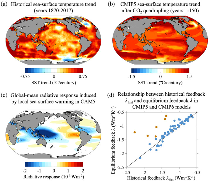
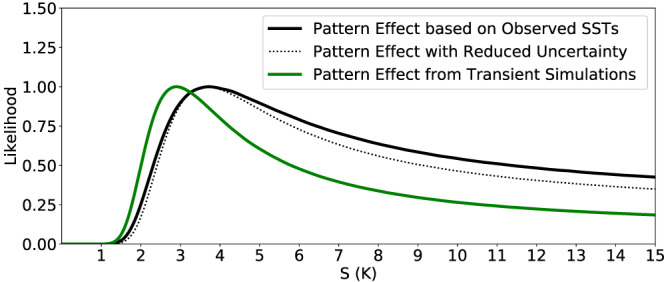
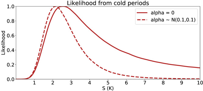
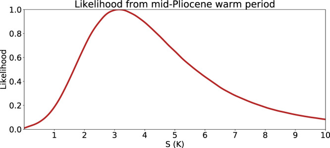
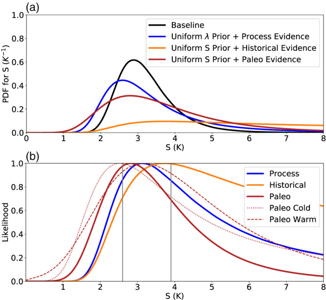
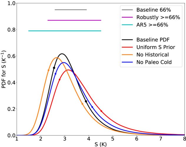
We assess evidence relevant to Earth's equilibrium climate sensitivity per doubling of atmospheric CO₂, characterized by an effective sensitivity S. This evidence includes feedback process understanding, the historical climate record, and the paleoclimate record. An S value lower than 2 K is difficult to reconcile with any of the three lines of evidence. The amount of cooling during the Last Glacial Maximum provides strong evidence against values of S greater than 4.5 K. Other lines of evidence in combination also show that this is relatively unlikely. We use a Bayesian approach to produce a probability density function (PDF) for S given all the evidence, including tests of robustness to difficult-to-quantify uncertainties and different priors. The 66% range is 2.6-3.9 K for our Baseline calculation and remains within 2.3-4.5 K under the robustness tests; corresponding 5-95% ranges are 2.3-4.7 K, bounded by 2.0-5.7 K (although such high-confidence ranges should be regarded more cautiously). This indicates a stronger constraint on S than reported in past assessments, by lifting the low end of the range. This narrowing occurs because the three lines of evidence agree and are judged to be largely independent and because of greater confidence in understanding feedback processes and in combining evidence. We identify promising avenues for further narrowing the range in S, in particular using comprehensive models and process understanding to address limitations in the traditional forcing-feedback paradigm for interpreting past changes.

Keywords: Bayesian methods; Climate; climate sensitivity; global warming.

Figure 1

Relation of (a) other climate sensitivity metrics and (b) predicted warming by late this century, to S as defined in section 2.1. In (a), symbols show 15 LongRunMIP model estimates of the equilibrium warming per doubling of CO₂ (Rugenstein, Bloch‐Johnson, Gregory, et al., 2019), with small purple symbols showing equilibria in 4xCO₂ simulations and large black symbols equilibria in 2xCO₂ simulations. Blue filled circles show TCR from CMIP5 models. In (b), projected change in global mean temperature in 2079–2099 relative to 1986–2005, under the RCP8.5 (red), RCP4.5 (magenta), and RCP2.6 (cyan) scenarios, from 24 CMIP5 models. CMIP5 data are from Grose et al. (2018). For each set of points, a best linear fit is shown, with one standard deviation shown in gray shading (assumed homogeneous except for ECS where it is assumed to scale linearly with S); see section 7.4 for further details on fits.

Figure 2

A Bayesian network diagram showing the dependence relationships between main variables in the inference model. Circles show uncertain variables, whose PDFs are estimated; squares show evidence (random effects on the evidence would appear as a second “parent” variable for each square and are omitted for simplicity). Colors distinguish the three main lines of evidence and associated variables (blue = process, orange = historical, and red = paleoclimate). For paleoclimate, only one ∆F/∆T climate change pair is shown but two independent ones are considered (see section 5).

Figure 3

Assessed values of the 2xCO₂ effective radiative forcing (ERF) at the TOA. Orange bars represent stratospheric‐adjusted radiative forcing (SARF), tropospheric and surface albedo adjustments, and their sum (i.e., ERF). The error bar indicates the 5–95% ranges of the respective terms. Further decomposed components are presented for reference by blue bars based on Etminan et al. (2016) and Smith et al. (2018). The contribution from land surface warming has been excluded in the surface adjustment.

Figure 4

Estimates of global mean climate feedbacks from observations of interannual variability (blue triangles), from CMIP5 and CMIP6 model simulations of global warming in response to an abrupt CO₂ quadrupling (colored circles—orange: Vial et al., 2013; green: Caldwell et al., 2016; red: Colman & Hanson, 2017; and purple: Zelinka et al., 2020) and from this assessment (black squares). Error bars on climate model feedback estimates span the one standard deviation range across models. Observational estimates are derived using a combination of ERA‐Interim meteorological fields and CERES TOA radiative fluxes (Loeb et al., 2009) covering the period March 2000 to December 2010 (Dessler, 2013). Error bars on the observational estimates are 1‐sigma uncertainties, accounting for autocorrelation. Individual feedbacks are computed by multiplying temperature‐mediated changes in relevant fields by radiative kernels (Huang et al., 2017; Shell et al., 2008; Soden et al., 2008). Error bars on values from this assessment correspond to 1‐sigma uncertainties. Note that Planck feedback estimates are offset by 2.5 W m⁻² K⁻¹ from their actual values in order that they appear within the plot range.

Figure 5

Multimodel and zonal mean cloud diagnostics: (a) Mean cloud fraction (contours, every 5%) and warming response (shading), with stippling where at least 20 of the 25 contributing CMIP5 models agree on the sign of the response. (b) Intermodel standard deviation of cloud fraction response. (c) Total cloud feedback from all clouds and also partitioned into contributions from low (cloud top pressures >680 hPa) and other (“nonlow,” cloud top pressures <680 hPa) clouds. (d) Non‐low‐ and (e) low‐cloud feedback partitioned into amount, altitude, and optical‐depth responses to warming. Latitudes where at least 14 of the 18 contributing models agree on the sign of the feedback are plotted with a solid line. Feedbacks in (c)–(e) are calculated from abrupt4xCO₂ simulations of seven CMIP5 models and from equilibrium 2xCO2 simulations of 11 CMIP3 slab‐ocean models (see Zelinka et al., 2016, for details). Note that all plots use an area‐weighted latitude scale. Figure based upon Zelinka et al. (2016).

Figure 6

Local tropical low‐cloud feedbacks from observations, large‐eddy simulations, and global climate models from Klein et al. (2017). Each dot represents the feedback from an individual research study. The upper horizontal bar indicates the central estimate and 90% confidence interval for the feedback inferred in that study from the observations. The lower bar indicates the range of feedbacks simulated by global climate models. Note that our assessment reinterprets the upper horizontal bar into a likelihood statement assuming a uniform prior and with considering additional evidence (section 3.3.2).

Figure 7

Assessed values of individual cloud feedbacks and the total cloud feedback based upon process evidence. For individual cloud feedbacks, maximum likelihood values are shown by black diamonds and the widths of blue rectangles, with 2 times the 1‐sigma likelihood values shown by the width of the black uncertainty bars. For the total cloud feedback, the mean value of the PDF is shown by a black diamond and the width of the accompanying blue rectangle, with 2 times the PDF standard deviation shown by the width of the black uncertainty bar.

Figure 8

PDFs and likelihood functions based upon the assessment of individual climate feedbacks and the emergent constraint literature. (a) PDF for λ from combining evidence on individual feedbacks using the Baseline λ _i prior. (b) Emergent constraint likelihood for λ. Note that this likelihood is not a PDF. See section 3.6 for an explanation of how the parameters of this likelihood function were determined and why they differ from the parameters recorded in Table 2. (c) PDF for S from combining evidence on ∆F _2xCO2 and individual feedbacks using uniform λ _i priors.

Figure 9

Individual feedbacks in CMIP5 climate models (circular symbols) and inferred from observations (error bars along the y axis). The y axis displays relationships derived from natural variability at the interannual time scale using 100 years of preindustrial control simulations from CMIP5 climate models (Colman & Hanson, 2017) and using ~11 years of observations between March 2000 and December 2010 (Dessler, 2013). Error bars span the 1‐sigma uncertainties of the observed feedback estimates. The x axis displays the long‐term feedbacks from climate model simulations of the response to an abrupt quadrupling of CO₂ (Colman & Hanson, 2017). The black dashed line is the 1:1 line, whereas the short solid thick lines among the climate model points display the ordinary least squares linear regression lines between simulated interannual and long‐term feedbacks.

Figure 10

Prior and posterior PDFs of total (anthropogenic plus natural) ΔF (W m⁻²), comparing the 2006–2018 period with the 1861–1880 period. The black curve shows the prior forcing used in the Baseline calculation, which uses the unconstrained aerosol forcing based on Equation (8) from Bellouin et al. (2020). The green curve shows the extended AR5 aerosol forcing. The orange curve shows the posterior PDF produced when all prior PDFs are updated by all evidence used in the full Baseline calculation (see section 7), including process, historical, and paleoclimate evidence.

Figure 11

(a) Likelihood function for S _hist derived from the planetary energy budget of the 2006–2018 period compared to the 1861–1880 period. Different analyses are shown based on the alternative estimates in Table 5. The dashed line shows the impact of reducing the uncertainty in ΔT and ΔN by 90%. The gray line shows the impact of using the original Cowtan and Way (2014) blended data set that mixes surface air temperature observations with sea surface temperature observations. The orange line shows the impact of using 1850–1900 for the earlier period, while the red line shows the impact of using the AR5 aerosol forcing. (b) PDF of S _hist based on likelihood function in (a) combined with a uniform prior on S _hist (black line) and PDF derived directly from Equation 19 (green line).

Figure 12

Illustration of probability density functions from alternative, published approaches (as labeled). Tokarska, Schurer, et al. (2020) rely on an energy budget approach using the observed warming and ocean heat uptake attributed to greenhouse warming and is most directly comparable to our main approach. The solid line relies on a flat prior in S, the dashed line is directly sampled (see text; similar to green line in Figure 11), and the dotted line is the same as the solid line, but based on doubled variance of climate variability when deriving the attributed warming estimates. Johansson et al. (2015) and Skeie et al. (2018) results are based on time‐space analysis using simple climate model fits to observations and are also depicted for a uniform prior in S. Results suggest that use of time‐space patterns (either in simple model fits or deriving attributed surface and ocean warming) reduces the upper tail of climate sensitivity yet is affected by uncertainty in methods used, particularly if using simple models.

Figure 13

Illustration of the pattern effect. (a) Linear trend in observed sea surface temperatures (SSTs) over years 1870–2017 from the AMIP2 data set (Hurrell et al., 2008). (b) Linear trend in CMIP5 mean SSTs over 150 years following abrupt CO₂ quadrupling. (c) Global mean TOA radiative response induced by perturbing SSTs in one region at a time, calculated as anomalous TOA radiative fluxes in response to local SST perturbations in NCAR's Community Atmosphere Model Version 5 (CAM5) (Zhou et al., 2017; see also Dong et al., 2019, for comparison to CAM4). (d) Relationship between historical feedbacks λ _hist and the long‐term λ in coupled CMIP5 and CMIP6 models using values from analysis in Lewis and Curry (2018) and Dong et al. (2020) (blue points), respectively, and for atmosphere‐only simulations from Andrews et al. (2018) (orange points).

Figure 14

Likelihoods for S based on historical energy budget estimates accounting for pattern effects using different methods. The black curve shows the likelihood we use for our main analysis in section 7, which is based on feedback changes estimated using observed SST patterns (Andrews et al., 2018) but with inflated uncertainty to account for several considerations described in the text. The dotted black line shows the effect of halving the uncertainty in Δλ. The green line shows the likelihood accounting for feedback changes estimated from transient simulations of coupled climate models (Armour, 2017).

Figure 15

Likelihood arising from cold‐period evidence (solid line). Dashed line shows the likelihood that would arise if state dependence of λ were omitted (α = 0).

Figure 16

Likelihood arising for mPWP.

Figure 17

Likelihood arising for the Paleocene‐Eocene Thermal Maximum. The maximum likelihood value of around 2 K corresponds to a 5‐K warming and ~3xCO₂ change together with its accompanying CH₄ increase.

Figure 18

Analysis of mPWP and PETM results. Blue and green dashed lines are mPWP and PETM results as previously shown. Red line is joint likelihood obtained accounting for dependency as described in the text. As explained in section 5.3.2, the mPWP result is our proposed result.

Figure 19

Blue‐dashed is the cold periods' likelihood. Red dashed line is the warm periods' likelihood. Magenta solid line is the final combined likelihood from paleoclimate evidence.

Figure 20

Posterior PDF for S and comparison of lines of evidence. Panel (a) shows our Baseline posterior PDF for S in black and PDFs for each main line of evidence individually, where the process evidence is combined with a uniform λ prior, while the others are combined with a uniform prior on S. Panel (b) shows marginal likelihoods for S for the various lines of evidence used in the Baseline calculation: the individual‐feedback process evidence (section 3), the likelihood from historical evidence (section 4), and the likelihoods for past warm and cold climates from paleoclimate evidence plus their combined likelihood (section 5). All likelihoods are scaled to have a maximum value of unity. Vertical gray lines show the 66% range for the Baseline posterior for S.

Figure 21

Prior predictive distributions for (a) λ and (b) S. Our Baseline (UL, red) prior is uniform in six λ _i feedbacks, each ~U(−10, 10) W m⁻² K⁻¹, compared to an alternative prior (US, orange), which reweights the Baseline prior to be uniform in S from near 0 to 20 K.

Figure 22

Graphical summary of statistics of posterior PDFs for S. UL is the Baseline calculation with a uniform prior on λ and US has a uniform prior on S. The middle group shows the effect of removing various lines of evidence in turn. UL + EC shows the impact of including the effect of emergent constraints. The effect of substituting fat‐tailed distributions for some lines of evidence is also shown for the Baseline case.

Figure 23

PDFs of the warming by late this century, from our Baseline PDF of S. These warming PDFs are obtained by converting S to warming using the best linear fit and then convolving the induced PDF with Gaussian uncertainty, as shown by the shading in Figure 1b. Results from RCP6.0 employ data from Forster et al. (2013). Note that the warming is calculated relative to 1985–2005; approximate warming relative to preindustrial is shown at the top, based on 0.6‐K warming having occurred by 1985–2005. Warming was estimated using the difference of 20‐year means centered on the years 1995 or 2089.

Figure 24

PDFs of S in comparison with AR5. The Baseline PDF is shown in black, and its 66% range (2.6–3.9 K) in gray. Colored curves show PDFs from sensitivity tests which cover a range for S, which could plausibly arise given reasonable alternative assumptions or interpretations of the evidence, summarized by the magenta line (2.3–4.5 K). These are the Baseline case but with a uniform S prior (red), the Baseline without the Historical evidence (orange), and the Baseline case without the cold paleoclimate evidence (blue). The 66%‐or‐greater (“likely”) range from the most recent IPCC assessment (AR5) (1.5–4.5 K) is shown in cyan. Circles indicate 17th and 83rd percentile values.

References

1. Abe‐Ouchi, A. , Saito, F. , Kageyama, M. , Braconnot, P. , Harrison, S. P. , Lambeck, K. , Otto‐Bliesner, B. L. , Peltier, W. R. , Tarasov, L. , Peterschmitt, J.‐Y. , & Takahashi, K. (2015). Ice‐sheet configuration in the CMIP5/PMIP3 Last Glacial Maximum experiments. Geoscientific Model Development, 8, 3621–3637. 10.5194/gmd-8-3621-2015 - DOI
1. Albani, S. , Mahowald, N. , Perry, A. , Scanza, R. , Zender, C. , Heavens, N. , Maggi, V. , Kok, J. , & Otto‐Bleisner, B. (2014). Improved dust representation in the Community Atmosphere Model. Journal of Advances in Modeling Earth Systems, 6, 541–570. 10.1002/2013MS000279 - DOI
1. Aldrin, M. , Holden, M. , Guttorp, P. , Skeie, R. B. , Myhre, G. , & Berntsen, T. K. (2012). Bayesian estimation of climate sensitivity based on a simple climate model fitted to observations of hemispheric temperatures and global ocean heat content. Environmetrics, 23, 253–271.
1. Allen, M. R. , Dube, O. P. , Solecki, W. , F. Aragón‐Durand, F. , Cramer, W. , Humphreys, S. , Kainuma, M. , Kala, J. , Mahowald, N. , Mulugetta, Y. , Perez, R. , Wairiu, M. , & Zickfeld, K. (2018). Chapter 1: Framing and context In Masson‐Delmotte V. et al. (Eds.), Global warming of 1.5°C. An IPCC Special Report on the impacts of global warming of 1.5°C above pre‐industrial levels and related global greenhouse gas emission pathways, in the context of strengthening the global response to the threat of climate change, sustainable development, and efforts to eradicate poverty.
1. Andrews, T. , Andrews, M. B. , Bodas‐Salcedo, A. , Jones, G. S. , Kulhbrodt, T. , Manners, J. , et al. (2019). Forcings, feedbacks and climate sensitivity in HadGEM3‐GC3.1 and UKESM1. Journal of Advances in Modeling Earth Systems, 11, 4377–4394. 10.1029/2019MS001866 - DOI