High-dimensional dynamics of generalization error in neural networks

Abstract

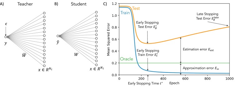
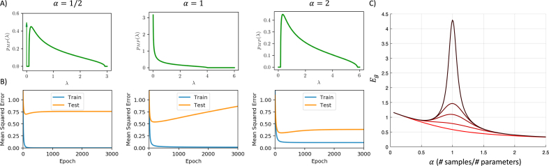
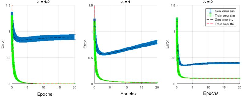
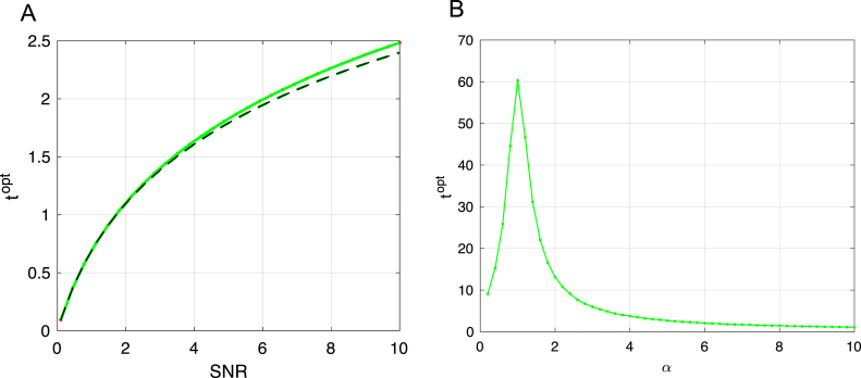
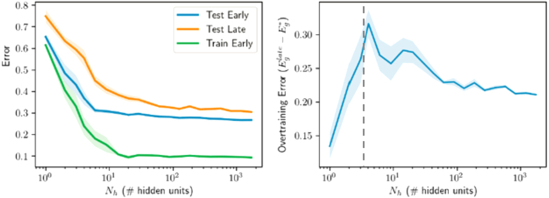
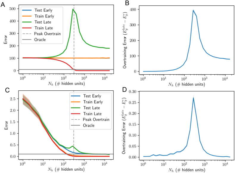
We perform an analysis of the average generalization dynamics of large neural networks trained using gradient descent. We study the practically-relevant "high-dimensional" regime where the number of free parameters in the network is on the order of or even larger than the number of examples in the dataset. Using random matrix theory and exact solutions in linear models, we derive the generalization error and training error dynamics of learning and analyze how they depend on the dimensionality of data and signal to noise ratio of the learning problem. We find that the dynamics of gradient descent learning naturally protect against overtraining and overfitting in large networks. Overtraining is worst at intermediate network sizes, when the effective number of free parameters equals the number of samples, and thus can be reduced by making a network smaller or larger. Additionally, in the high-dimensional regime, low generalization error requires starting with small initial weights. We then turn to non-linear neural networks, and show that making networks very large does not harm their generalization performance. On the contrary, it can in fact reduce overtraining, even without early stopping or regularization of any sort. We identify two novel phenomena underlying this behavior in overcomplete models: first, there is a frozen subspace of the weights in which no learning occurs under gradient descent; and second, the statistical properties of the high-dimensional regime yield better-conditioned input correlations which protect against overtraining. We demonstrate that standard application of theories such as Rademacher complexity are inaccurate in predicting the generalization performance of deep neural networks, and derive an alternative bound which incorporates the frozen subspace and conditioning effects and qualitatively matches the behavior observed in simulation.

Keywords: Generalization error; Neural networks; Random matrix theory.

Fig. 1

Learning from a noisy linear teacher. (A) A dataset $\mathcal{D}=\{x^{\mu },y^{\mu }\},\mu =1,\dots ,P$ of $P$ examples is created by providing random inputs $x$ to a teacher network with a weight vector $\overline{w}$, and corrupting the teacher outputs with noise of variance ${\sigma }_{ϵ}^2$. (B) A student network is then trained on this dataset $\mathcal{D}$. (C) Example dynamics of the student network during full batch gradient descent training. Training error (blue) decreases monotonically. Test error, also referred to as generalization error, (yellow), here computable exactly (4), decreases to a minimum $E_g^{\ast }$ at the optimal early stopping time $t^{\ast }$ before increasing at longer times ($E_g^{\text{late}}$), a phenomenon known as overtraining. Because of noise in the teacher’s output, the best possible student network attains finite generalization error (“oracle”, green) even with infinite training data. This error is the approximation error $E_{\infty }$. The difference between test error and this best-possible error is the estimation error $E_{\text{est}}$. (For interpretation of the references to color in this figure legend, the reader is referred to the web version of this article.)

Fig. 2

The Marchenko–Pastur distribution and high-dimensional learning dynamics. (A) Different ratios of number training samples ($P$) to network parameters ($N$) ($\alpha =\frac{P}{N}$) yield different eigenvalue densities in the input correlation matrix. For large $N$, this density is described by the MP distribution (15), which consists of a ‘bulk’ lying between $[{\lambda }_{-},{\lambda }_{+}]$, and, when $\alpha <1$, an additional delta function spike at zero. When there are fewer samples than parameters ($\alpha <1$, left column), some fraction of eigenvalues are exactly zero (delta-function arrow at origin), and the rest are appreciably greater than zero. When the number of samples is on the order of the parameters ($\alpha =1$, center column), the distribution diverges near the origin and there are many nonzero but arbitrarily small eigenvalues. When there are more samples than parameters ($\alpha >1$, right column), the smallest eigenvalues are appreciably greater than zero. (B) Dynamics of learning. From (13), the generalization error is harmed most by small eigenvalues; and these are the slowest to be learned. Hence for $\alpha =1∕2$ and $\alpha =2$, the gap in the spectrum near zero protects the dynamics from overtraining substantially (eigenvalues which are exactly zero for $\alpha =1∕2$ are never learned, and hence contribute a finite error but no overtraining). For $\alpha =1$, there are arbitrarily small eigenvalues, and overtraining is substantial. (C) Plot of generalization error versus $\alpha$ for several training times, revealing a clear spike near $\alpha =1$. Other parameters: $N=100,\text{INR}=0,\text{SNR}=5$. As the colors vary from red to black the training time increases $\frac{t}{\tau }=[5,20,50,100,1000]$. (For interpretation of the references to color in this figure legend, the reader is referred to the web version of this article.)

Fig. 3

Generalization and training error dynamics compared with simulations. Here we demonstrate that our theoretical predictions for generalization and training error dynamics at different measurement densities ($\alpha =1∕2,\alpha =1$, and $\alpha =2$) match with simulations. The simulations for generalization (blue) and training (green) errors have a width of $\pm 2$ standard deviations generated from 20 trials using $N=300$, $P=\alpha N$ and Gaussian input, noise, and parameters with ${\sigma }_{\overline{w}}=1,{\sigma }_w^0=0$, and $\text{SNR}=5$. The simulations show excellent agreement with our theoretical predictions for generalization and training error provided in (14), (26). (For interpretation of the references to color in this figure legend, the reader is referred to the web version of this article.)

Fig. 4

Impact of data quality and dimensionality on optimal stopping time. In (A) we plot the impact of SNR on the optimal stopping time with low measurement density $\alpha =.05$, and compare this to the predictions of (16) with $\lambda =1$ because the non-zero values of the MP distribution are highly peaked around this value at low measurement density. In (B) we plot the impact of measurement density on the optimal stopping time in the low noise (SNR $=$ 100) limit, where longer training is required near $\alpha =1$ because the high quality of the data makes it beneficial to learn weights even in the small eigenvalue directions. In both plots green curves are optimal stopping time numerical predictions computed via gradient descent on $t$ using (14). (For interpretation of the references to color in this figure legend, the reader is referred to the web version of this article.)

Fig. 5

Optimal stopping performance. In (A) we plot the generalization error from early stopping (red stars) versus optimal quadratically regularized regression (blue line). In this example there is no more than 3 percent relative error between the two, which peaks near $\alpha =1$ when the spectrum of non-zero eigenvalues is broader. In (B) we plot generalization error vs. $\alpha$ for different initial weight norms. In the limited data regime, small initial weights are crucial for good generalization. In both plots, we have fixed SNR $=$ 5 and ${\sigma }_{\overline{w}}^2=1$ which implies that even at large measurement density $\alpha$ the generalization error asymptotes to a non-zero value due to noise $0.2=\frac{1}{\text{SNR}}$.

Fig. 6

Reduction of deep linear network dynamics. (A) The student network is a deep linear network of depth $D+1$. (B-D) Comparisons of simulations of the full generalization dynamics for networks initialized with small weights (gold) to simulations of the reduced dynamics (green) for different depths and parameter settings. Training error in blue. (For interpretation of the references to color in this figure legend, the reader is referred to the web version of this article.)

Fig. 7

Learning from a nonlinear teacher. (A) The teacher network ($N_t$ ReLUs). (B) The student network ($N_h$ ReLUs, but only the output weights are trained). (C) Effect of model complexity. Optimal early stopping errors as a function of number of hidden units $N_h$ for the case $\text{SNR}=1,\text{INR}=0,N_i=15,N_t=30$ and $P=300$ training samples. Shaded regions show $\pm 1$ standard error of the mean over 50 random seeds. (D) Overtraining peaks at an intermediate level of complexity near the number of training samples: when the number of free parameters in the student network equals the number of samples (300). (E) The eigenspectrum of the hidden layer of a random non-linear neural network with $P=1000$ samples and an $N_i=100$ dimensional input space. We consider three cases and find a similar eigenvalue density to a rescaled Marchenko–Pastur distribution when we concentrate only on the small eigenvalues and ignore a secondary cluster of $N_i$ eigenvalues farther from the origin. Left: Fewer hidden nodes than samples ($N_h=500$ hidden units) leads to a gap near the origin and no zero eigenvalues. Center: An equal number of hidden nodes and samples ($N_h=1000$) leads to no gap near the origin so that eigenvalues become more probable as we approach the origin. Right: More hidden nodes than samples ($N_h=2000$) leads to a delta function spike of probability 0.5 at the origin with a gap to the next eigenvalue. (F) Average training dynamics for several models illustrating overtraining at intermediate levels of complexity. (For interpretation of the references to color in this figure legend, the reader is referred to the web version of this article.)

Fig. 8

Training directly on data: two layer ReLU network trained on binary MNIST classification of 7s vs. 9s with 1024 training samples. First layer weights of student are random and fixed. The less pronounced peak is likely due to computational restrictions which limited training time and maximum model size (see text).

Fig. 9

Two layer network generalization error decomposition: Here we use data generated from a two layer teacher network with ReLU activations, 20 hidden units, and no noise. The student network has fixed random first layer weights and ReLU activations. (A) Shows the approximation error in blue, the null-space error in red, the over-fitting error in gold, and the sum of all three in cyan. Generalization error computed from 5000 new examples are black error bars. Plus sign denotes generalization error with a two layer teacher with $w_{\parallel }^{\ast }$ weights and Gaussian noise with a variance matched to the sum of approximation and null-space error. The number of examples used in training is $P=50$ (dashed vertical line) and number of trails used to compute error bars is 500. (B) Shows the approximation error (blue) and null space error (red) as well as the sum of the two (dashed black). (For interpretation of the references to color in this figure legend, the reader is referred to the web version of this article.)

Fig. 10

Impact of label noise on performance of wide networks: We plot the generalization error decomposition as in Fig. 9 for (A) an under-parameterized $N_h=10$ and (B) an over-parameterized $N_h=200$ network. Because output noise is added to both networks, approximation of the function is difficult even for the larger network because the function it is learning is not deterministic. However, the fitting error is larger in the larger network due to the eigenvalue spectrum of the hidden layer covariance. This is in contrast to our finding that larger networks perform better in the deterministic, low noise setting depicted in Fig. 9. Other parameters: $P=50$, $N_t=20$, ${\sigma }_w^0=0$, ${\sigma }_{\overline{w}}=1$.

Fig. 11

Impact of initialization on performance of wide networks. We plot the generalization error decomposition as in Fig. 9 for (A) an under-parameterized $N_h=10$ and (B) an over-parameterized $N_h=200$ network. We demonstrate that large initializations have a detrimental impact on generalization performance in wide neural networks which are over-parameterized and not on smaller networks. This effect is due to the frozen subspace observed when training with fewer examples than free parameters, and again is in contrast to our finding that larger networks perform better in the low initialization setting depicted in Fig. 9. Other parameters: $P=50$, $N_t=20$, ${\sigma }_{ϵ}=0$, ${\sigma }_{\overline{w}}=1$.

Fig. 12

Training both layers of nonlinear student. These simulations are of the same setting as that of Fig. 7, but with both layers of the student network trained. The number of hidden units for which the total number of free parameters is equal to the number of samples ($N_h+N_i{N}_h=P$) is marked with a dashed line and aligns well with the peak in overtraining observed. (For interpretation of the references to color in this figure legend, the reader is referred to the web version of this article.)

Fig. 13

Two layer network trained (without frozen weights) on binary MNIST classification of 7s vs. 9s with 1024 training samples. The qualitative trends identified earlier hold: over-training is a transient phenomenon at intermediate levels of complexity, and large models work well: no over-fitting is observed given optimal early stopping. Note that the over-training is less distinct than before primarily because these experiments were run for only 5000 epochs as opposed to tens of thousands of epochs as in Fig. 7, Fig. 12, due to computational constraints.

Fig. 14

Memorization, generalization, and $\text{SNR}$. Nonlinear ReLU networks with fixed first layer (same setting as Fig. 7) are trained on target labels of varying $\text{SNR}$. (A-B) Nearly random target labels ($\text{SNR}=0.01$). In the high dimensional regime in which the model size outstrips the number of examples (here $N_h>300$, indicated by vertical dotted line), all networks easily attain zero training error when trained long enough, thereby showing the ability to memorize an arbitrary dataset. (C-D) These exact same model sizes, however, generalize well when applied to data with nearly noise-free labels ($\text{SNR}=10$). In fact in the low noise regime, even early stopping becomes unnecessary for large enough model sizes. The dynamics of gradient descent naturally protect generalization performance provided the network is initialized with small weights, because directions with no information have no dynamics. (For interpretation of the references to color in this figure legend, the reader is referred to the web version of this article.)

References

1. Advani M., Ganguli S. An equivalence between high dimensional bayes optimal inference and m-estimation. Advances in Neural Information Processing Systems. 2016
1. Advani M., Ganguli S. 2016. Statistical mechanics of high dimensional inference supplementary material. In: See https://ganguli-gang.stanford.edu/pdf/HighDimInf.Supp.pdf.
1. Advani M., Ganguli S. Statistical mechanics of optimal convex inference in high dimensions. Physical Review X. 2016;6(3)
1. Advani M., Lahiri S., Ganguli S. Statistical mechanics of complex neural systems and high dimensional data. Journal of Statistical Mechanics: Theory and Experiment. 2013;(03):P03014.
1. Amari S., Murata N., Müller K.R. Statistical theory of overtraining - Is cross-validation asymptotically effective? Advances in Neural Information Processing Systems. 1996
LinkOut - more resources