Clouds and Convective Self-Aggregation in a Multimodel Ensemble of Radiative-Convective Equilibrium Simulations

Abstract

The Radiative-Convective Equilibrium Model Intercomparison Project (RCEMIP) is an intercomparison of multiple types of numerical models configured in radiative-convective equilibrium (RCE). RCE is an idealization of the tropical atmosphere that has long been used to study basic questions in climate science. Here, we employ RCE to investigate the role that clouds and convective activity play in determining cloud feedbacks, climate sensitivity, the state of convective aggregation, and the equilibrium climate. RCEMIP is unique among intercomparisons in its inclusion of a wide range of model types, including atmospheric general circulation models (GCMs), single column models (SCMs), cloud-resolving models (CRMs), large eddy simulations (LES), and global cloud-resolving models (GCRMs). The first results are presented from the RCEMIP ensemble of more than 30 models. While there are large differences across the RCEMIP ensemble in the representation of mean profiles of temperature, humidity, and cloudiness, in a majority of models anvil clouds rise, warm, and decrease in area coverage in response to an increase in sea surface temperature (SST). Nearly all models exhibit self-aggregation in large domains and agree that self-aggregation acts to dry and warm the troposphere, reduce high cloudiness, and increase cooling to space. The degree of self-aggregation exhibits no clear tendency with warming. There is a wide range of climate sensitivities, but models with parameterized convection tend to have lower climate sensitivities than models with explicit convection. In models with parameterized convection, aggregated simulations have lower climate sensitivities than unaggregated simulations.

Keywords: climate sensitivity; cloud feedbacks; clouds; convection; radiative‐convective equilibrium; self‐aggregation.

Figure 1

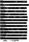
Time series of domain‐mean outgoing longwave radiation (OLR; W m⁻²) in the RCE_small300 (left column) and RCE_large300 simulations (right column). The top row shows GCM simulations with parameterized convection, with the single‐column version of the model in (a) and the global model in (b). The middle row shows simulations with explicit convection (c, d), including CRM, LES, and GCRM simulations. The bottom row shows the WRF‐GCM simulations with 50 km resolution and parameterized convection. The black vertical line to the left of each plot is a 25 W m⁻² scale bar, but the absolute values of OLR and distance between the curves has no meaning here, as the curves are offset for visual clarity according to OLR + ⟨OLR⟩ + i*x x, where ⟨ ⟩ is the ensemble mean, i is the model index (according to alphabetical order), and xx = 2 for RCE_large and xx = 10 for RCE_small.

Figure 2

Hourly‐averaged outgoing longwave radiation (W m⁻²) at Day 80 of the RCE_small300 simulation for all cloud‐resolving models. Each panel displays a different model and the size of each panel represents the domain size, which varies slightly across models.

Figure 3

Hourly averaged outgoing longwave radiation (W m⁻²) at Day 80 of the RCE_small300 (a, d, g, j, m, p, s) and RCE_small_vert300 (b, e, h, k, n, q, t) simulations and Day 50 of the RCE_small_les300 (c, f, l, o, r, u) simulations for CM1, DALES, DALES‐damping, ICON_LEM, MESONH, MicroHH, and SAM. The size of each panel represents the domain size, which varies slightly across models. DALES and DALES‐damping have larger values of OLR because the radiative properties of ice clouds were erroneously configured. DALES‐damping‐rad is a corrected version, shown for reference (note that it is the RCE_small_vert300 simulation that is shown in panel (i) despite it being in the column with LES simulations).

Figure 4

Hourly averaged outgoing longwave radiation (W m⁻²) at Day 80 of the RCE_large300 simulation for all cloud‐resolving models. Each panel displays a different model and the size of each panel represents the domain size, which varies slightly across models. Note that FV3 is missing from the figure because outgoing longwave radiation was only reported as daily averages.

Figure 5

Hourly averaged outgoing longwave radiation (W m⁻²) at Day 80 of the RCE_large300 simulation for all global models (except for IPSL‐CM6, which reported daily averaged output). All models shown are GCMs with parameterized convection (panels a–k) except MPAS, NICAM, and SAM (panels l–n), which are global cloud‐resolving models that employ reduced Earth radius of R_E/8, R_E/4, and R_E/4, respectively, and are shown to scale and, in the box, zoomed in.

Figure 6

Hourly averaged outgoing longwave radiation (W m⁻²) at Day 80 of the RCE_large300 simulation for all versions of WRF 3.5.1. Panel (a) displays the same WRF‐COL‐CRM configuration as in Figure 4l. The other panels (b–h) show WRF‐GCM in the Cartesian RCE_large300 configuration but with 50 km grid spacing and convective parameterizations.

Figure 7

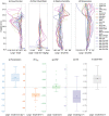
Horizontal‐mean temperature profile, averaged in time excluding the first 75 days of simulation of the RCE_small (top row: a–d) and RCE_large (bottom row: e–h) simulations at 300 K. The first column (a, e) includes all models that performed each type of simulation, where the black line is the ensemble mean, the blue shading shows the range across all models, and the orange lines indicate the interquartile range (IQR). The other columns display the temperature anomaly in each subgroup of models as an anomaly from the ensemble mean of that subgroup, for models with parameterized convection (second column: b, f), CRMs (third column: c, g), models that performed RCE_small_vert (dashed) and RCE_small_les (solid) simulations (panel d; RCE_small_les simulations are averaged over Days 25–50), and GCRMs (panel h).

Figure 8

Horizontal‐mean relative humidity profile, averaged in time excluding the first 75 days of simulation of the RCE_small (top row a–d) and RCE_large (bottom row: e–h) simulations at 300 K. The first column (a, e) includes all models that performed each type of simulation, where the black line is the ensemble mean, the blue shading shows the range across all models, and the orange lines indicate the interquartile range (IQR). The other columns display each subgroup of models: models with parameterized convection (second column: b, f), CRMs (third column: c, g), models that performed RCE_small_vert (dashed) and RCE_small_les (solid) simulations (panel d; RCE_small_les simulations are averaged over Days 25–50), and GCRMs (panel h).

Figure 9

Domain‐wide cloud fraction profile, averaged in time excluding the first 75 days of simulation of the RCE_small (top row: a–d) and RCE_large (bottom row: e–h) simulations at 300 K. The first column (a, e) includes all models that performed each type of simulation, where the black line is the ensemble mean, the blue shading shows the range across all models, and the orange lines indicate the interquartile range (IQR). The other columns display each subgroup of models: models with parameterized convection (second column: b, f), CRMs (third column: c, g), models that performed RCE_small_vert (dashed) and RCE_small_les (solid) simulations (panel d; RCE_small_les simulations are averaged over Days 25–50), and GCRMs (panel h).

Figure 10

Horizontal‐mean total cloud water condensate profile, averaged in time excluding the first 75 days of simulation of the RCE_small (top row: a–d) and RCE_large (bottom row: e–h) simulations at 300 K. The first column (a, e) includes all models that performed each type of simulation, where the black line is the ensemble mean, the blue shading shows the range across all models, and the orange lines indicate the interquartile range (IQR). The other columns display each subgroup of models: models with parameterized convection (second column: b, f), CRMs (third column: c, g), models that performed RCE_small_vert (dashed) and RCE_small_les (solid) simulations (panel d; RCE_small_les simulations are averaged over Days 25–50), and GCRMs (panel h).

Figure 11

Box and whiskers plots of domain‐average quantities, averaged in time excluding the first 75 days of the RCE_small300 and RCE_large300 simulations. RCE_small_vert300 and RCE_small_les300 simulations are included in the “Small” statistics. The top row (panels a–e) includes all models in the statistics while the bottom row (panels f–j) splits the models into those with explicit (“S_E” and “L_E”) and parameterized convection (“S_P” and “L_P”), where the “S” and “L” indicate small and large simulations, respectively. The variables shown are precipitation rate (mm day⁻¹; panels a and f), net radiation at the top of atmosphere (R_TOA; W m⁻², downward defined as positive; panels b and g), condensed water path (CWP; mm; panels c and h), precipitable water (PW; kg m⁻²; panels d and i), and the tropospheric lapse rate (K km⁻¹; panels e and j). The asterisk indicates the multimodel mean, the horizontal line the median, the shaded region the interquartile range, and the circles the outliers. The whiskers are defined as 1.5 times the interquartile range; this does not extend beyond the range of the data.

Figure 12

Degree of aggregation in RCE_large300 based on subsidence fraction (red circles), I_org (blue squares), and spatial variance of column relative humidity (green triangles) in all models, averaged in time excluding the first 75 days of simulation. The models are ordered such that the models with explicit convection are to the left of the dashed line and models with parameterized convection are to the right of the dashed line. Within each group of models, they are ordered according to their values of subsidence fraction. The two models for which subsidence fraction could not be computed are listed first. Box plots indicate the spread of each metric across all models.

Figure 13

Horizontal and time mean (average excluding the first 75 days) of the difference between pairs of RCE_small300 and RCE_large300 simulations, for cloud fraction (a), total cloud water (b), relative humidity (c), temperature (d), precipitation rate (e), net radiation at the top of the atmosphere (f), condensed water path (g), precipitable water (h), and the tropospheric lapse rate (i). The difference is taken as RCE_large300‐RCE_small300. In the box and whiskers plots (e–i), the asterisk indicates the multimodel mean, the horizontal line the median, the shaded region the interquartile range, and the open circles the outliers. The whiskers are defined as 1.5 times the interquartile range; this does not extend beyond the range of the data.

Figure 14

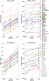
Horizontal‐ and time‐mean height (a, c) and temperature (b, d) at the location of the domain‐wide anvil cloud peak as a function of SST in the RCE_small simulations (a, b) and RCE_large simulations (c, d). The dashed lines are linear regression lines of best fit.

Figure 15

Domain‐wide anvil cloud fraction as a function of SST in the RCE_small simulations (a, b) and RCE_large simulations (c, d). The left panels (a, c) show the actual value of the anvil cloud fraction while the right panels (b, d) show the value of the anvil cloud fraction as an anomaly from its value in the simulation at 300 K. The dashed lines are linear regression lines of best fit.

Figure 16

The rate of change of the aggregation metrics per degree K in the RCE_large simulations based on I_org (blue squares), subsidence fraction (red circles), and spatial variance of column relative humidity (green triangles) in all models, based on the difference between simulations at 295 and 305 K. The models are ordered such that the models with explicit convection are to the left of the dashed line and models with parameterized convection are to the right of the dashed line. Within each group of models, they are ordered according to their values of df_sub/dSST. The two models for which subsidence fraction could not be computed (due to missing output) are listed first. Box plots indicate the spread of each metric's rate of change across models, with outlier indicated with symbols.

Figure 17

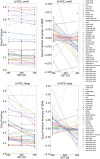
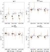
Net climate feedback parameter λ = dR_TOA/dT (a), change in cloud radiative effect λ_cloud = dCRE/dT (b), change in shortwave cloud radiative effect ${\lambda }_{\text{cloud}}^{\text{SW}}=dCR{E}_{SW}/dT$ (c), and change in longwave cloud radiative effect ${\lambda }_{\text{cloud}}^{\text{LW}}=dCR{E}_{LW}/dT$ (d). RCE_large simulations are shown in filled symbols; RCE_small simulations are shown in open symbols. Averages over all models are shown in black, averages over models with parameterized convection are shown in red, and averages over models with explicit convection are shown in blue. The feedbacks are calculated over 295–300, 295–305, and 300–305 K, as indicated on the x axis. The error bars indicate the interquartile range.

References

1. Arnold, N. P. , & Randall, D. A. (2015). Global‐scale convective aggregation: Implications for the Madden‐Julian Oscillation. Journal of Advances in Modeling Earth Systems, 7, 1499–1518. 10.1002/2015MS000498 - DOI
1. Bazile, E. , Couvreux, F. , Moigne, P. L. , Genthon, C. , Holtslag, A. A. M. , & Svensson, G. (2014). GABLS4: An intercomparison case to study the stable boundary layer over the Antarctic plateau. Global Energy Water Cycle Experiment News, 24(4), 4–4.
1. Becker, T. , Hohenegger, C. , & Stevens, B. (2017). Imprint of the convective parameterization and sea‐surface temperature on large‐scale convective self‐aggregation. Journal of Advances in Modeling Earth Systems, 9, 1488–1505. 10.1002/2016MS000865 - DOI
1. Becker, T. , & Stevens, B. (2014). Climate and climate sensitivity to changing CO2 on an idealized land planet. Journal of Advances in Modeling Earth Systems, 6, 1205–1223. 10.1002/2014MS000369 - DOI
1. Blossey, P. N. , Bretherton, C. S. , & Wyant, M. C. (2009). Subtropical low cloud response to a warmer climate in a superparameterized climate model. Part II: Column modeling with a cloud resolving model. Journal of Advances in Modeling Earth Systems, 1, 8 10.3894/JAMES.2009.1.8 - DOI