Hamiltonian modelling of macro-economic urban dynamics

Abstract

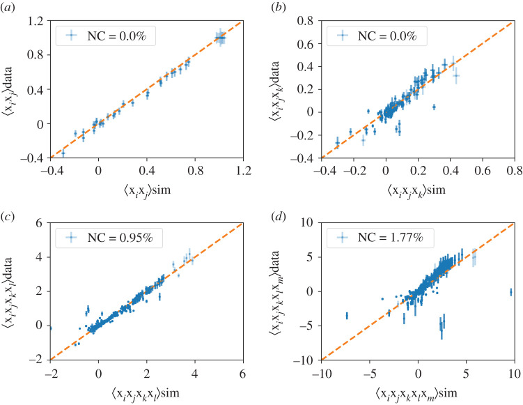
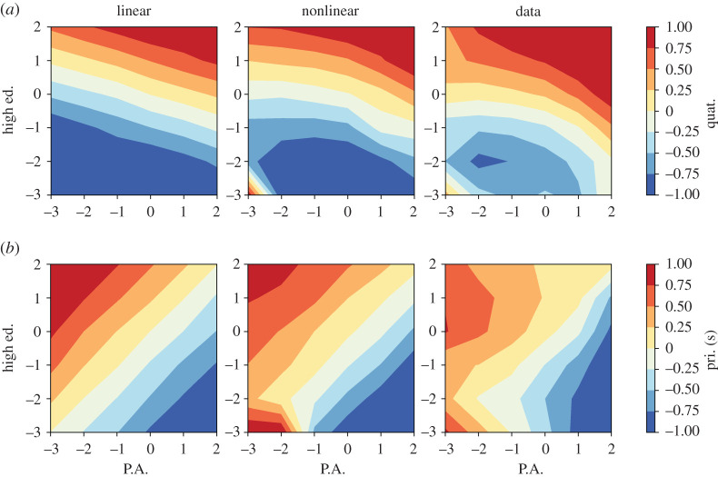
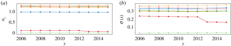
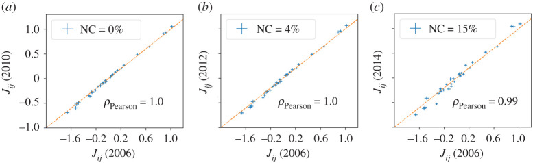
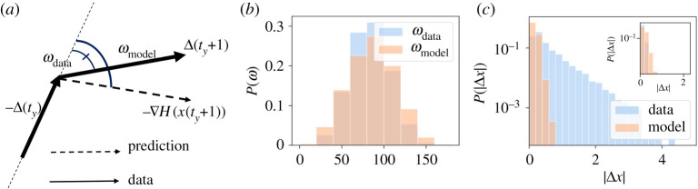
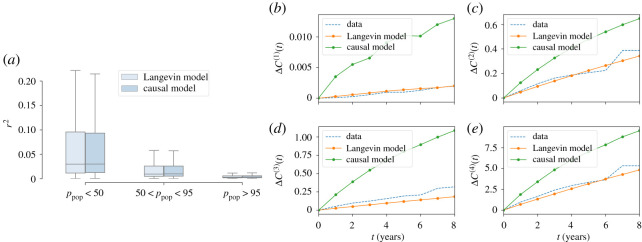
The rapid urbanization makes the understanding of the evolution of urban environments of utmost importance to steer societies towards better futures. Many studies have focused on the emerging properties of cities, leading to the discovery of scaling laws mirroring the dependence of socio-economic indicators on city sizes. However, few efforts have been devoted to the modelling of the dynamical evolution of cities, as reflected through the mutual influence of socio-economic variables. Here, we fill this gap by presenting a maximum entropy generative model for cities written in terms of a few macro-economic variables, whose parameters (the effective Hamiltonian, in a statistical-physical analogy) are inferred from real data through a maximum-likelihood approach. This approach allows for establishing a few results. First, nonlinear dependencies among indicators are needed for an accurate statistical description of the complexity of empirical correlations. Second, the inferred coupling parameters turn out to be quite robust along different years. Third, the quasi time-invariance of the effective Hamiltonian allows guessing the future state of a city based on a previous state. Through the adoption of a longitudinal dataset of macro-economic variables for French towns, we assess a significant forecasting accuracy.

Keywords: maximum entropy; scaling; urban indicators.

Figure 1.

Comparisons between the correlators of order 2 (a), 3 (b), 4 (c) and 5 (d) obtained with the empirical data of year 2012 (y-axis) and the Hamiltonian model (equation (2.3)) (x-axis). We report the percentage of components of each correlation which is not compatible with the data via a t-test with p-value 0.05 (see electronic supplementary material, S6).

Figure 2.

Rescaled indicators for Jobs in Quaternary Sector (a) and Jobs in Primary and Secondary Sectors (b) as functions of the rescaled indicators for Jobs in Public Administration (x-axis) and Fraction of highly educated people (y-axis). Areas in red (blue) represent communes with a large (small) value of the rescaled indicator used as dependent variable. The first column (with the label linear) reports the results obtained with the Hamiltonian model without the terms J⁽¹⁾ and J⁽³⁾. The second column (with the label nonlinear) reports the results obtained with the complete model of equation (2.3). The last column reports the results obtained by binning the points for the communes in the year (2012).

Figure 3.

(a) Scaling exponents a_i for the socio-economic indicators i as a function of time. (b) σ(x_i) for the socio-economic indicators i as a function of time. Each indicator is represented by a different colour.

Figure 4.

Comparisons between the J⁽²⁾ parameters of different years (2006–2010 in (a), 2006–2012 in (b), 2006–2014 in (c)). The dotted line represents the relation of equality (i.e. the diagonal of the first half-plane in the Cartesian space. The percentage of non-compatible (NC) reported refers to the percentage of components that cannot be considered as equal with a t-test and a threshold p-value of 0.05.

Figure 5.

(a) Graphical representation of the angles ω_data (the smaller angle in (a)) and ω_model (the larger angle in (a)), identified respectively by the variation Δ(t_y+1) at time t_y and the predicted variation of the model at the same time $-\mathrm{\nabla }H(\mathbf{x}(t_y))$, and by the two subsequent variations Δ(t_y) and Δ(t_y+1). (b) Comparison between the angle ω_data between the velocity of the system at consecutive times and the angle ω_model between the velocity of the system and the velocity predicted by equation (2.5). (c) Variations Δx_i(t_y) for all the components i of the feature vector in the same two cases. In the inset, we show the same comparison excluding communes with a population larger than 10⁴.

Figure 6.

(a) Distribution of r² computed according to equation (2.7) and with a causal inference model, inferred using temporal information explicitly. The values of r² have been divided according to the percentile of the commune population distribution. (c,b,d,e) Evolution of the distance between macroscopic observables computed in different years with respect to those computed in 2012 (t = 0 on the x-axis).

References

1. Bettencourt LM. 2013. The origins of scaling in cities. Science 340, 1438–1441. (10.1126/science.1235823) - DOI - PubMed
1. Bettencourt L, Lobo J, Youn H. 2013. The hypothesis of urban scaling: formalization, implications and challenges. (http://arxiv.org/abs/1301.5919).
1. Bettencourt LM, Lobo J, Strumsky D, West GB. 2010. Urban scaling and its deviations: revealing the structure of wealth, innovation and crime across cities. PLoS ONE 5, e13541 (10.1371/journal.pone.0013541) - DOI - PMC - PubMed
1. Youn H, Bettencourt LM, Lobo J, Strumsky D, Samaniego H, West GB. 2016. Scaling and universality in urban economic diversification. J. R. Soc. Interface 13, 20150937 (10.1098/rsif.2015.0937) - DOI - PMC - PubMed
1. Batty M. 2008. The size, scale, and shape of cities. Science 319, 769–771. (10.1126/science.1151419) - DOI - PubMed