Power-law population heterogeneity governs epidemic waves

Abstract

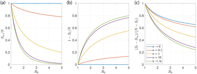
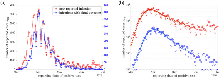
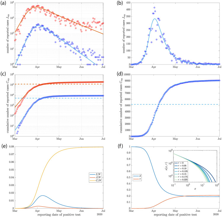
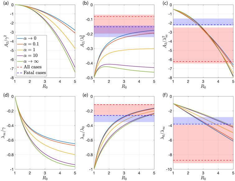
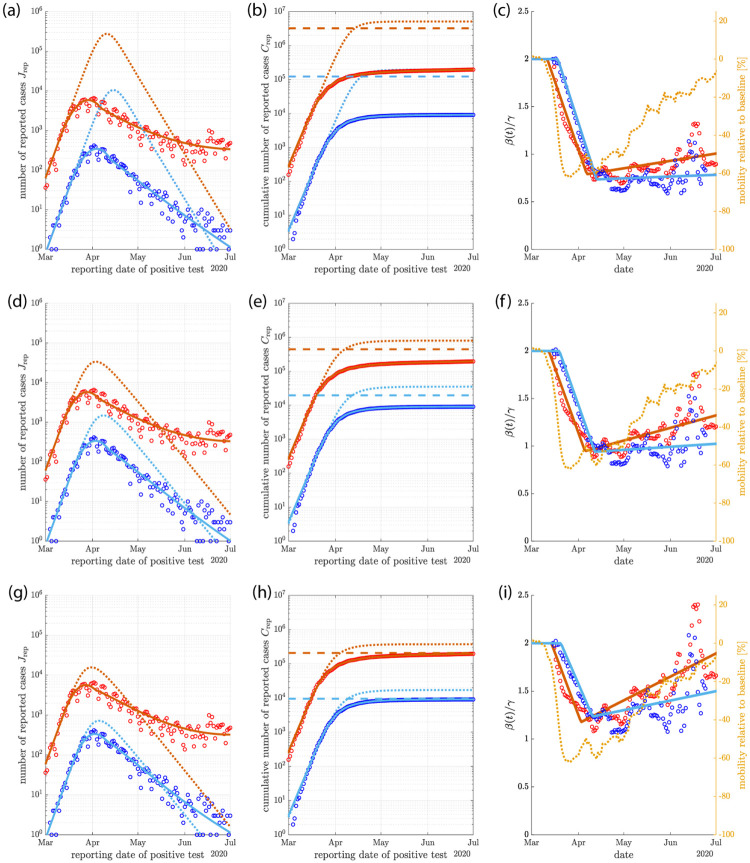
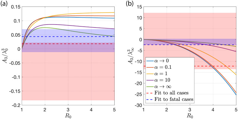
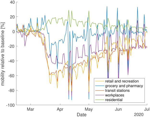
We generalize the Susceptible-Infected-Removed (SIR) model for epidemics to take into account generic effects of heterogeneity in the degree of susceptibility to infection in the population. We introduce a single new parameter corresponding to a power-law exponent of the susceptibility distribution at small susceptibilities. We find that for this class of distributions the gamma distribution is the attractor of the dynamics. This allows us to identify generic effects of population heterogeneity in a model as simple as the original SIR model which is contained as a limiting case. Because of this simplicity, numerical solutions can be generated easily and key properties of the epidemic wave can still be obtained exactly. In particular, we present exact expressions for the herd immunity level, the final size of the epidemic, as well as for the shape of the wave and for observables that can be quantified during an epidemic. In strongly heterogeneous populations, the herd immunity level can be much lower than in models with homogeneous populations as commonly used for example to discuss effects of mitigation. Using our model to analyze data for the SARS-CoV-2 epidemic in Germany shows that the reported time course is consistent with several scenarios characterized by different levels of immunity. These scenarios differ in population heterogeneity and in the time course of the infection rate, for example due to mitigation efforts or seasonality. Our analysis reveals that quantifying the effects of mitigation requires knowledge on the degree of heterogeneity in the population. Our work shows that key effects of population heterogeneity can be captured without increasing the complexity of the model. We show that information about population heterogeneity will be key to understand how far an epidemic has progressed and what can be expected for its future course.

Fig 1. Effects of population heterogeneity on the dynamics of SIR models.

Examples for the time course of fraction of susceptible S/N (green), fraction of infected I/N (orange) and fraction of the cumulative number of infected C/N (blue) in a SIR model with N total individuals. (a)-(c) Homogeneous SIR model with R₀ = 2.5 and γ = 0.13 day⁻¹. (d)-(f) Heterogeneous SIR model with same R₀ and γ and with α = 0.1. (a) and (d) show time course as linear plot, (b) and (e) show semi logarithmic plots of the same variables. (c) and (f) show the normalized time dependent reproduction number R(t)/R₀ (yellow) and the average susceptibility $\overline{x}\left(t\right)$ (purple) as a function of time. The dotted lines in (a),(b),(d) and (e) indicate the herd immunity level C_I. Other parameters: N = 810⁷ individuals and I₀ = 10 initially infected.

Fig 2. Fraction of susceptible individuals at long times.

(a) Fraction S_∞/N of susceptible individuals that remain at long times as a function of the basic reproduction number R₀ for different degrees of population heterogeneity characterized by the values of α. The limit α → ∞ corresponds to the classic case with homogeneous populations (green). In the limit α → 0 populations are most heterogeneous (blue). (b) Fraction S_I/N of susceptible individuals as a function of R₀ at the peak where the number of infected is maximal for different α. (c) Ratio of infections after the peak S_m − S_∞ and infections before the peak N − S_m as a function of R₀.

Fig 3

(a) Daily new SARS-CoV-2 infections reported in the early months of 2020 in Germany. The number of new reported infections per day $J_{\text{rep}}^t$ (red symbols) is shown together with the number of reported infections per day for those cases with later fatal outcome $J_{\text{rep}}^f$ (blue symbols). (b) Semi logarithmic representation of the same data. The dashed and solid lines represent linear and cubic fits to the data in specific time intervals. They are used to estimate the initial and final growth rates λ₀ and λ_∞ as well as $A_2=\ddot{J}/J$ and $A_3=\stackrel{⃛}{J}/J$ at the maximum of the rate of new cases J_max. We find λ₀ ≃ 0.269 day⁻¹ (0.336 day⁻¹), λ_∞ ≃ −0.068 day⁻¹ (−0.038 day⁻¹), A₂ ≃ −10⁻² day⁻² (−0.9110⁻² day⁻²) and A₃ ≃ 6.810⁻⁴ day⁻³ (7.510⁻⁴ day⁻³) for the fatal cases (for all reported cases).

Fig 4. Time course of the SARS-CoV-2 epidemic in Germany (symbols) compared to solutions of the heterogeneous SIR model (lines).

(a) and (b) Data on daily reported infections (red) and on reported infections with later fatal outcome (blue) as logarithmic and linear plots. (c) and (d) same data and model solutions as in (a) and (b) but for cumulative numbers of cases. The horizontal dashed lines indicate scaled herd immunity levels. Parameter values for the model solution are R₀ = 2.67 (R₀ = 3.91), γ = 0.146 (γ = 0.069), α = 0.05 and N = 810⁷ for the fatal cases (for all cases). The case fatality rate that corresponds to this solution is f = 0.13% (f = 0.11%). (e) Time courses of the fraction of infected I/N (blue), the new cases per day J/N (red) and the fraction of cumulative cases C/N (yellow) for R₀ = 2.67 and γ = 0.146. (f) Time course of the average susceptibility $\overline{x}={(R/R_0)}^{1/(1+\alpha )}$ (blue), where R is the time dependent reproduction number and of $\tau =\alpha (1/\overline{x}-1)$ (red) for the solution shown in (e). Inset: distributions of susceptibility in the population for different values of τ.

Fig 5. Role of population heterogeneity for the behavior of the generalized SIR model.

Plots of various dimensionless ratios of parameters characterizing the shape of the infection wave for different values of α. Here the limit α → ∞ corresponds to the homogeneous SIR model, the limit α → 0 to the strongly heterogeneous case. Here λ₀ and λ_∞ denote the initial and final growth rate, $A_2=\ddot{J}/J$ and $A_3=\stackrel{⃛}{J}/J$ describe the shape of the wave at the maximum of new cases per day J. The horizontal dashed lines correspond to estimates from fits shown in Fig 3, the shaded regions indicate uncertainty ranges, see Appendix D.

Fig 6. Scenarios of mitigation.

(a)-(c) Early mitigation by strong reduction of β for a homogeneous population (large α limit). The new cases per day are shown in (a) as symbols. A fit of the mitigated model is shown as solid lines. The solution for same parameter values R₀ = 2 and γ = 0.24 but without mitigation is shown as dotted lines. The corresponding cumulative numbers of cases are shown in (b). Herd immunity levels corresponding to these solutions are indicated as horizontal dashes lines. The time dependence of β(t) are shown in (c) as solid lines. The time courses of β inferred from the data is shown as symbols. Mobility data indicating social activities in Germany relative to baseline values are shown in orange for comparison. (d)-(f) same plots as in (a)-(c) but for a moderate mitigation and heterogeneous population with R₀ = 2, γ = 0.24 and α = 0.1. (g)-(i) Heterogeneous population with mild mitigation and release leading to almost herd immunity. Red symbols and lines correspond to the case of all reported infections, blue data and lines correspond to reported infections of fatal cases.

Fig 7. Normalized coefficient A3=J⃛/J at the peak of new cases per day.

(a) The ratio $A_3/{\lambda }_0^3$ as a function of R₀ is shown for different values of α. (b) The ratio $A_3/{\lambda }_{\infty }^3$ as a function of R₀ for the same values of α. The dashed lines represent the values inferred from the data shown in Fig 3 for all cases (red) and fatal cases (blue). The shaded colored regions correspond to the uncertainties of the fits to the data.

Fig 8. Mobility changes for a representative set of commonly visited places in Germany up to July 1 2020 from [34].

References

1. Murray J. D. Mathematical Biology Interdisciplinary Applied Mathematics. Springer, New York, 3rd ed edition, 2002.
1. Daley Daryl J and Gani J. M. Epidemic Modelling: An Introduction. Cambridge University Press, 1999.
1. Hethcote Herbert W. The Mathematics of Infectious Diseases. SIAM Review, 42(4):599–653, January 2000. 10.1137/S0036144500371907 - DOI
1. O. Diekmann, Hans Heesterbeek, and Tom Britton. Mathematical Tools for Understanding Infectious Diseases Dynamics. Princeton Series in Theoretical and Computational Biology. Princeton University Press, Princeton, 2013.
1. Brownlee J. Historical note on Farr’s theory of the epidemic. BMJ, 2(2850):250–252, August 1915. 10.1136/bmj.2.2850.250 - DOI - PMC - PubMed
Publication types