The Geometry of Abstraction in the Hippocampus and Prefrontal Cortex

Abstract

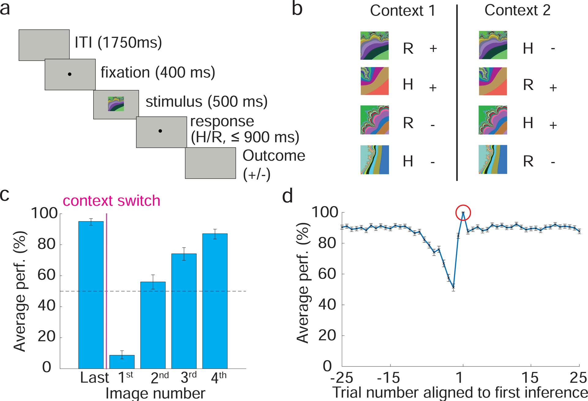
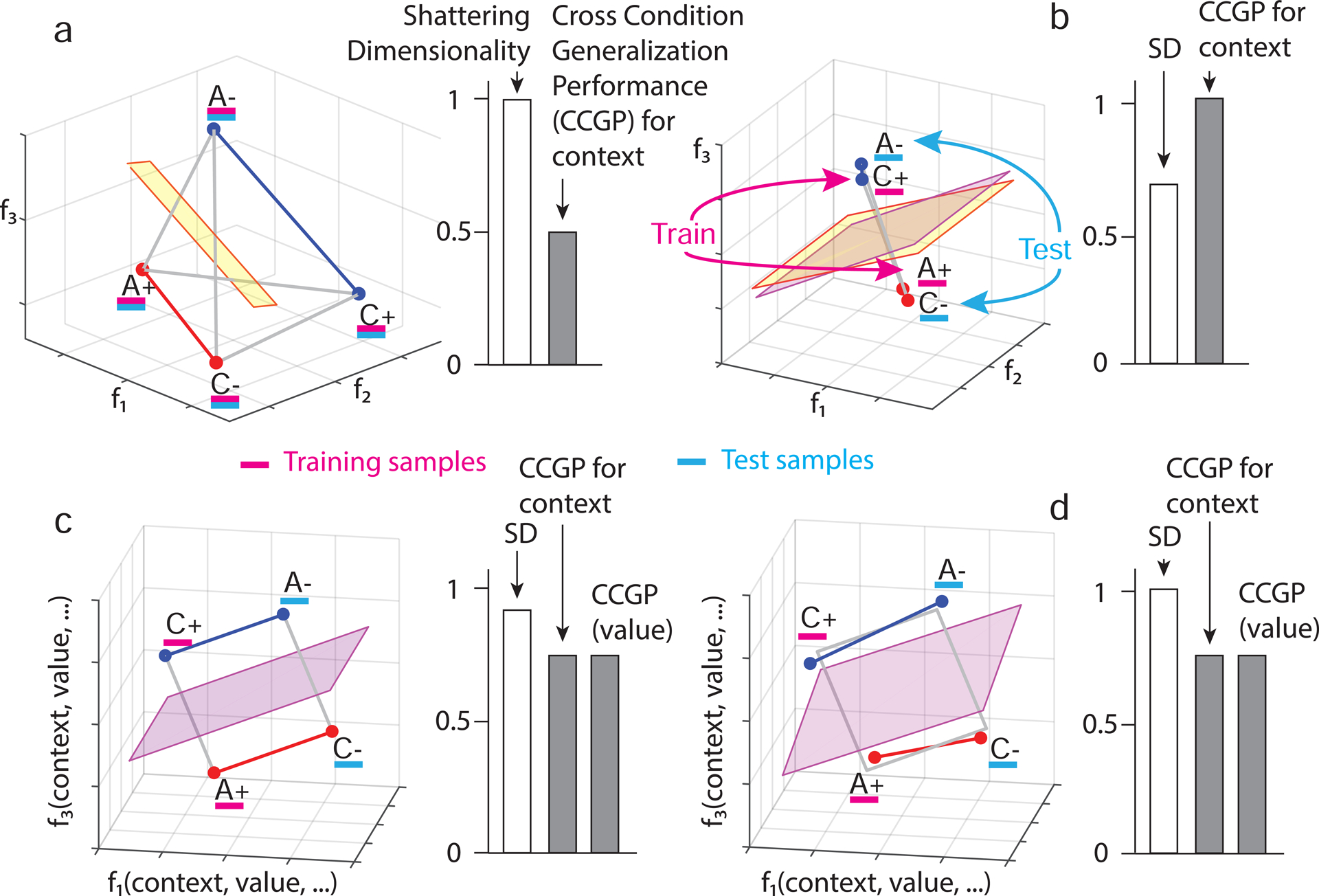
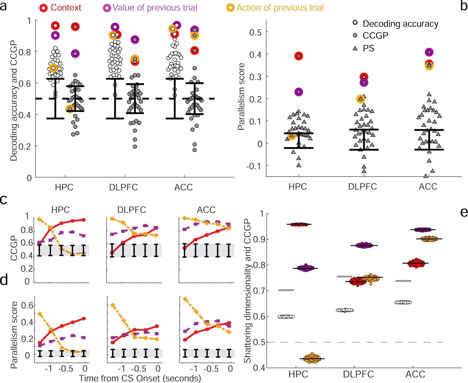
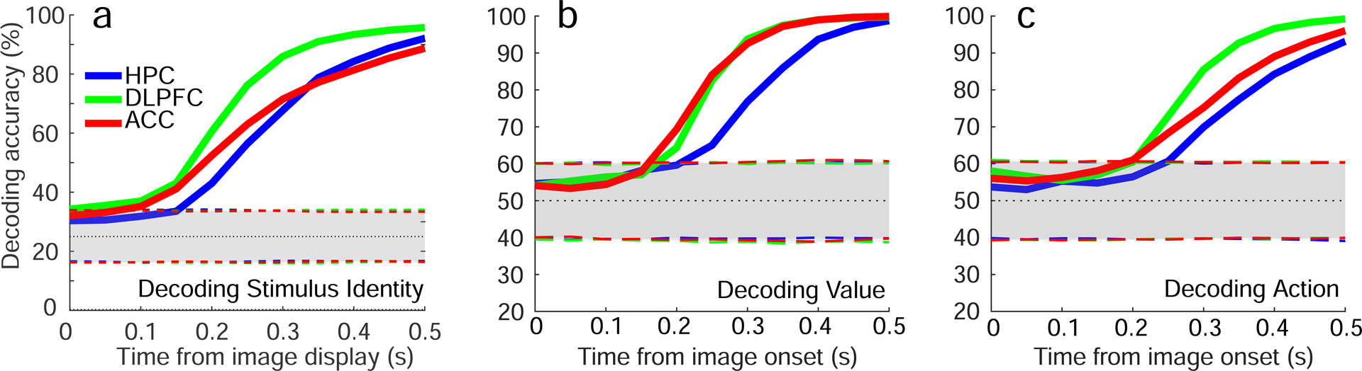
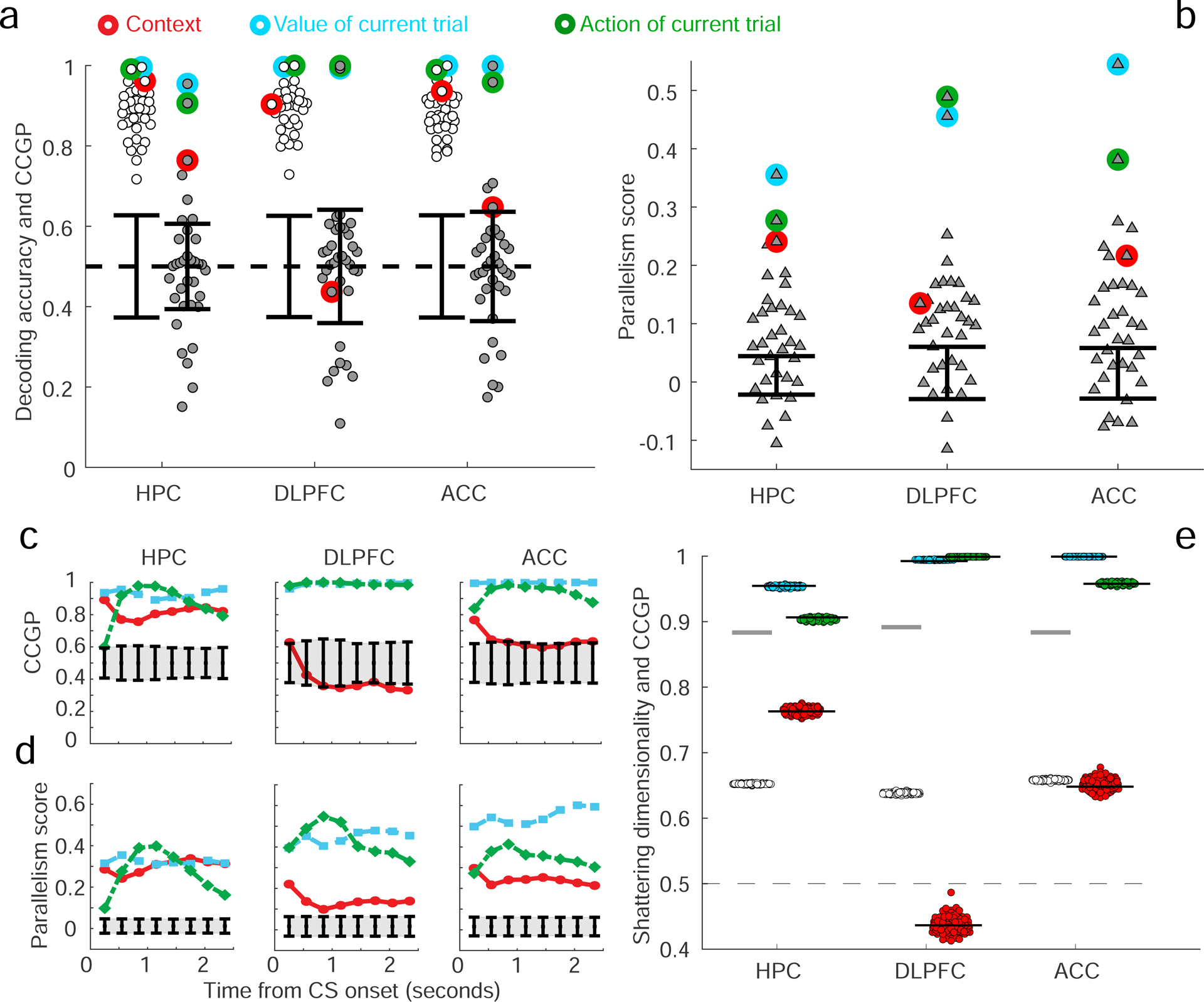
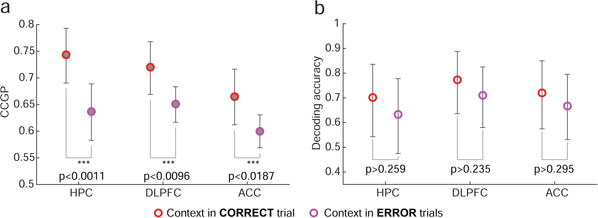
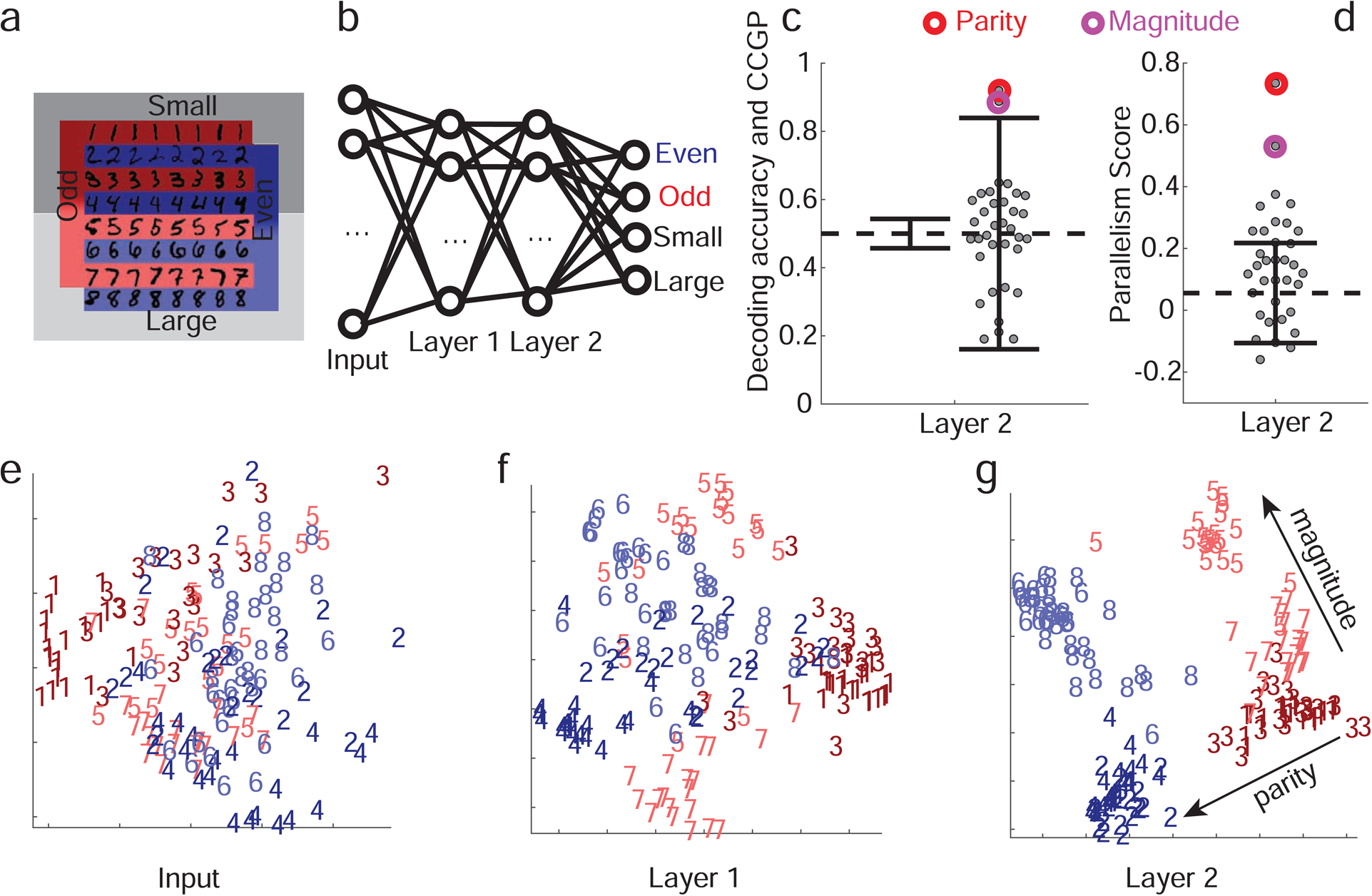
The curse of dimensionality plagues models of reinforcement learning and decision making. The process of abstraction solves this by constructing variables describing features shared by different instances, reducing dimensionality and enabling generalization in novel situations. Here, we characterized neural representations in monkeys performing a task described by different hidden and explicit variables. Abstraction was defined operationally using the generalization performance of neural decoders across task conditions not used for training, which requires a particular geometry of neural representations. Neural ensembles in prefrontal cortex, hippocampus, and simulated neural networks simultaneously represented multiple variables in a geometry reflecting abstraction but that still allowed a linear classifier to decode a large number of other variables (high shattering dimensionality). Furthermore, this geometry changed in relation to task events and performance. These findings elucidate how the brain and artificial systems represent variables in an abstract format while preserving the advantages conferred by high shattering dimensionality.

Keywords: abstraction; anterior cingulate cortex; artificial neural networks; dimensionality; disentangled representations; factorized representations; hippocampus; mixed selectivity; prefrontal cortex; representational geometry.

Figure 1:. Task and behavior.

a. Sequence of events within a trial. A monkey holds down a button, then fixates and views one of 4 familiar fractal images. A delay interval ensues, during which the operant response must be indicated (release or continue to hold the button, H and R). After a trace period, a liquid reward is delivered for correct responses for 2 of the 4 stimuli. Correct responses to the other 2 stimuli result in no reward, but avoids a timeout and trial repetition. b. Task scheme, SRO mappings for conditions in the 2 contexts. A-D, stimuli. +/−, reward/no reward for correct choices. Operant and reinforcement contingencies are orthogonal. After 50–70 trials in one context, context switches; experiments contain many context switches. c. Monkeys utilize inference to adjust behavior. Average percent correct plotted for the first presentation of the last image appearing before a context switch (”Last”) and for the first instance of each image after a context switch (1–4). For image numbers 2–4, monkeys adjusted performed at above chance despite not having experienced these trials in the current context (inference). Binomial parameter estimate, bars are 95% Clopper-Pearson confidence intervals d. Average percent correct performance plotted vs. trial number aligned on the first correct trial where the monkey used inference (red circle, defined as the first correct trial among the first presentations of the 2nd, 3rd or 4th image type appearing after a context switch). So if Image 1 is the first image after a context switch, and the first presentation of image 2 is performed correctly, it is the first correct inference trial. If it is performed incorrectly, the first correct inference trial could occur on the first presentation of image 3 or 4.

Figure 2:. The geometry of abstraction.

Different representations of context can have distinct geometries, each with different generalization properties. Each panel depicts in the firing rate space points that represent the average firing rate of 3 neurons in only 4 of the 8 conditions from experiments. The 4 conditions are labeled according to stimulus identity (A,C) and reward value (+,−). a. A random representation (points are at random locations in the firing rate space), which allows for decoding of context. The yellow plane represents a linear decoder that separates the 2 points of context 1 (red) from the 2 points of context 2 (blue). The decoder is trained on a subset of trials from all conditions (purple) and tested on held out trials from the same conditions (cyan) (see Figure S1a for more details). All other variables corresponding to different dichotomies of the 4 points can also be decoded using a linear classifier; hence the shattering dimensionality (SD) is maximal, but CCGP is at chance (right histogram). b. Abstraction by clustering: points are clustered according to context. A linear classifier is trained to discriminate context on rewarded conditions (purple). Its generalization performance (CCGP) is tested on unrewarded conditions not used for training (cyan). The separating plane when trained on rewarded conditions (purple) is different from the one obtained when all conditions are used for training (yellow), but for this clustered geometry, both planes are very similar. With clustered geometry, CCGP is maximal for context, but context is also the only variable encoded. Hence, SD is close to chance (right histogram). (See Methods S2 Clustering index as a measure of abstraction). Notice that the form of generalization CCGP involves is different from traditional decoding generalization to held out trials (see Methods S3 Relation between CCGP and decoding performance in classification tasks). c. Multiple abstract variables: factorized/disentangled representations. The 4 points are arranged on a square. Context is encoded along the direction parallel to the two colored segments, and value is in the orthogonal direction. In this arrangement, CCGP for both context and value are high; the SD is high but not maximal because the combinations of points that correspond to an exclusive OR (XOR) are not separable. Individual neurons exhibit linear mixed selectivity (see Methods S6 Selectivity and abstraction in a general linear model of neuronal responses). d. Distorted square: a sufficiently large perturbation of the points makes the representation higher dimensional (points no longer lie on a plane); a linear decoder can now separate all possible dichotomies, leading to maximal SD, but at the same time CCGP remains high for both value and context. See Methods S5 The trade off between dimensionality and our measures of abstraction and Fig. S2 that constructs geometries that have high SD and CCGP at the same time.

Figure 3:. Decoding accuracy, CCGP and parallelism score (PS) in the 3 recorded brain areas.

A-b. CCGP, decoding accuracy and PS for the variables that correspond to all 35 dichotomies shown separately for each brain area in a 900 ms time epoch beginning 800 ms before image presentation. The points corresponding to the context, value and action of the previous trial are highlighted with circles of different colors. Table T2 contains the values of CCGP and PS for all dichotomies. Context and value are represented in an abstract format in all 3 brain areas, but action is abstract only in PFC (although it can be decoded in HPC (see also Fig. S4 to visualize the arrangement of the points in the firing rate space). Almost all dichotomies can be accurately decoded, and the SD is high: HPC, 0.70; DLPFC, 0.75; ACC, 0.74 (see also Methods S4 PCA Dimensionality of the neural representations, which describes other measures of dimensionality). Error bars are ± two standard deviations around chance level as obtained from a geometric random model (CCGP) or from a shuffle of the data (decoding accuracy and PS). Results were qualitatively similar in the 2 monkeys (see Figure S5). c-d. CCGP (c) and the PS (d) plotted as a function of time for the variables context, action and value in the 3 brain areas (900 ms window stepped in 300 ms increments; last window ends at 100 ms after stimulus onset, before a visual response occurs). e. Measured SD in each brain area is significantly greater than the SD of a perfectly factorized representation. To determine if a perfectly factorized representation, which typically has high CCGP, is consistent with the high SD observed in experimental data, a perfectly factorized null model is constructed by placing the centroids of the noise clouds that represent the 8 different experimental conditions at the vertices of a cuboid. The lengths of the sides of the cuboid are tuned to reproduce (on average) the CCGP values observed in the experiment for the variables context, value, and action. From this artificially generated data corresponding to a perfectly factorized model, SD and CCGP are calculated, with the procedure repeated 100 times for each brain area. SD (empty circles) and CCGP for the variables context, value and action (colored circles) plotted for each realization of the random model. Gray horizontal lines, SD from the experiments; black horizontal lines, CCGP for context, value and action, mimicking experimental data shown in a. The factorized models re-capitulate the recorded CCGP values, but the SD values measured in all 3 brain areas are significantly higher than in any realization of the factorized model. The difference between the experimentally measured SD and the average SD of the factorized model is more than an order of magnitude larger than the standard deviation of the model SD distribution in all cases, indicating that the experimental data is not consistent with such a factorized geometry.

Figure 4:. Decoding accuracy for stimulus, value and action.

Decoding accuracy for stimulus identity, value and action plotted as a function of time in the 3 brain areas. Decoding of stimulus identity employs a 4-way classifier, so chance is 0.25. The use of a linear decoder was employed because neural responses are highly heterogeneous, exhibiting mixed selectivity (see Fig. S3a) and are rarely specialized (see Fig. S6). Dotted line, chance. Shaded areas, two-sided 95%-confidence intervals calculated with a permutation test (randomly shuffling trials, 1,000 repetitions). See Figure S3 for decoding of task relevant variables across a longer timescale).

Figure 5:. Decoding accuracy, CCGP and the PS after stimulus onset in the 3 brain areas.

a,b. CCGP, decoding accuracy and PS for all 35 dichotomies in the time interval from 100ms to 1000ms after stimulus onset. See Table T2 for the values of CCGP and PS for all dichotomies. Error bars, ± 2 standard deviations around chance as obtained from a geometric random model (CCGP) or from a shuffle of the data (decoding accuracy and PS). The SD is higher in this interval than in the earlier time epoch: HPC 0.88, DLPFC 0.89 and ACC 0.88. Results were qualitatively similar in the two monkeys (see Figs. S5). C-d. CCGP (c) and the PS (d) plotted as a function of time for the variables context, action and value in the 3 brain areas (900 ms window beginning 100 ms after stimulus onset, 300 ms steps). e. The SD observed in each brain area is significantly greater than the SD of a perfectly factorized representation. Same analysis as in Figure 3e but for this later time interval.

Figure 6:. The relationship between CCGP for context and behavioral performance.

a. CCGP for context, measured in the 900 ms time interval ending 100 ms after stimulus onset, is significantly lower on error trials than on correct trials in all 3 brain areas. Average decreases (± one standard deviation) in CCGP on error trials are: 0.107 ± 0.038 (p<0.0011) in HPC, 0.0691±0.0303 (p<0.0096) in DLPFC, and 0.0651±0.0309 (p<0.0187) in ACC (average, standard deviation and p-values computed over 10,000 repetitions of bootstrap re-sampling trials using a sub-population of 180 neurons per area; error bars, 95th percentiles of the bootstrap distributions). Since errors occurred in a relatively small fraction of all trials, neurons were selected according to a different criterion than other analyses, resulting in fewer neurons being included in this analysis (see Methods). Results in this figure and Figure 3 are thus not directly comparable. b. Decoding accuracy for context is not significantly different for correct and error trials. Average drops (± one standard deviation) of decoding accuracy between correct and error trials: 0.069±0.108 (p≥0.259) in HPC, 0.0627±0.0903 (p≥0.235) in DLPFC, and 0.0532±0.0984 (p<0.295) in ACC (averages, standard deviations, p-values and error bars obtained analogously as in (a) on the same neurons). See Methods and Table T1 for details.

Figure 7:. Simulations of a multi-layer neural network replicate experimentally observed geometry.

a. Schematic of the two discrimination tasks using the MNIST dataset and color code for panels e,f,g. The colors indicate parity, and shading indicates the magnitude of the digits (darker for smaller ones). b. Diagram of the network architecture. The input layer receives images of MNIST handwritten digits 1–8. The two hidden layers have 100 units each, and in the final layer there are 2 pairs of output units corresponding to 2 binary variables. The network is trained using back-propagation to simultaneously classify inputs according to whether they depict even/odd and large/small digits. c. CCGP and decoding accuracy for variables corresponding to all 35 balanced dichotomies when the second hidden layer is read out. Only the 2 dichotomies corresponding to parity and magnitude are significantly different from a geometric random model (chance level: 0.5; the two solid black lines indicate ±2standard deviations). Decoding performance is high for all dichotomies, and hence inadequate to identify the variables stored in an abstract format. d. Same as b, but for the PS, with error bars (±2 standard deviations) obtained from a shuffle of the data. Both CCGP and the PS allow us to identify the output variables used to train the network. e-g. Two-dimensional MDS plots of the representations of a subset of images in the input (pixel) space (e), as well as in the first (f) and second hidden layers (g). In the input layer there is no structure apart from the accidental similarities between the pixel images of certain digits (e.g. ones and sevens). In the first, and even more so in the second, layer, a clear separation between digits of different parities and magnitudes emerges in a geometry with consistent and approximately orthogonal coding directions for the two variables. For neural network simulations of the task performed by the monkeys, See Methods S1 Simulations of the parity/magnitude task: dependence on hyperparameters for more details. See also Methods S8 Deep neural network models of task performance, Figure S7 for a reinforcement learning model, and Figure S8 for a supervised learning model.

References

1. Antzoulatos EG & Miller EK (2011), ‘Differences between neural activity in prefrontal cortex and striatum during learning of novel abstract categories’, Neuron 71(2), 243–249. - PMC - PubMed
1. Barak O, Rigotti M & Fusi S (2013), ‘The sparseness of mixed selectivity neurons controls the generalization-discrimination trade-off.’, The Journal of neuroscience : the official journal of the Society for Neuroscience 33, 3844–3856. - PMC - PubMed
1. Barto AG & Mahadevan S (2003), ‘Recent advances in hierarchical reinforcement learning’, Discrete Event Dynamic Systems 13(4), 341–379.
1. Behrens TE, Muller TH, Whittington JC, Mark S, Baram AB, Stachenfeld KL & Kurth-Nelson Z (2018), ‘What is a cognitive map? organizing knowledge for flexible behavior’, Neuron 100(2), 490–509. - PubMed
1. Bellman RE (1957), Dynamic Programming., Princeton University Press.
Publication types