Integration of geoscience frameworks into digital pathology analysis permits quantification of microarchitectural relationships in histological landscapes

Abstract

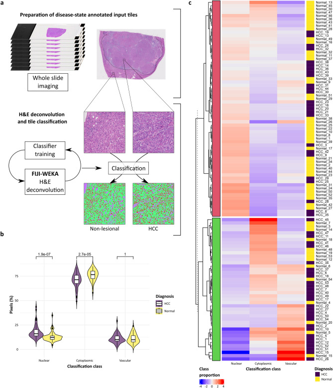
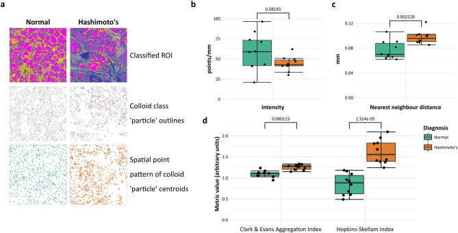
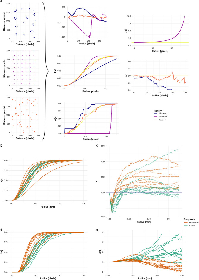
Although gold-standard histological assessment is subjective it remains central to diagnosis and clinical trial protocols and is crucial for the evaluation of any preclinical disease model. Objectivity and reproducibility are enhanced by quantitative analysis of histological images but current methods require application-specific algorithm training and fail to extract understanding from the histological context of observable features. We reinterpret histopathological images as disease landscapes to describe a generalisable framework defining topographic relationships in tissue using geoscience approaches. The framework requires no user-dependent training to operate on all image datasets in a classifier-agnostic manner but is adaptable and scalable, able to quantify occult abnormalities, derive mechanistic insights, and define a new feature class for machine-learning diagnostic classification. We demonstrate application to inflammatory, fibrotic and neoplastic disease in multiple organs, including the detection and quantification of occult lobular enlargement in the liver secondary to hilar obstruction. We anticipate this approach will provide a robust class of histological data for trial stratification or endpoints, provide quantitative endorsement of experimental models of disease, and could be incorporated within advanced approaches to clinical diagnostic pathology.

Figure 1

Fully classified histological images can be considered categorical maps and analysed as part of a fully computational pipeline using landscape ecology and geosciences methodologies. (a) Categorical representations of the landscape are routinely evaluated in landscape ecology and geosciences by specific tools. The generation of a fully segmented output image from a histological input, by any available method, is an analogous process differing only in scale (Contains modified Copernicus Sentinel data 2019 processed by Sentinel Hub under CC BY 4.0. Mapped tiles copyright OpenStreetMap contributors under Open Database Licence). (b) A pipeline using fully segmented images converts the images to an appropriate file format feeding the landscapemetrics package in R, generating the complete suite of metrics described in FRAGSTATS, and other holistic landscape measures of complexity and organisation.

Figure 2

Standard pixel counts of classified image are limited value alone. (a) A dataset of 54 whole slide images of H&E-stained sections from liver resections for hepatocellular carcinoma were used as an exemplar for the added value derived by landscape analysis of classified images. Lesional (HCC) and non-lesional fields were selected from each slide and a simple WEKA machine-learning H&E deconvolution classifier trained to allow pixel classification of tiles into 3 classes (nuclear, cytoplasm, vascular channels). (b) Pixel-class proportions for ‘nuclear’ and ‘cytoplasmic’ were significantly different between HCC and non-lesional regions when analysed by group (violin plot with kernel density and median (centre line), first and third quartiles (lower and upper box limits), 1.5 × interquartile range (whiskers); p-values of unpaired two-sided two-sample t-test for each metric, n = 54). (c) K-means clustering using these three pixel-class proportions alone was poor at segregating regions by diagnosis.

Figure 3

Classification-agnostic landscape metrics allow histopathological phenotyping in human disease and represent an intuitive input dataset for machine-learning disease-classification methods. (a) Individual complexity metrics from non-lesional liver and hepatocellular carcinoma can be used as discrete phenotyping measures (violin plot with kernel density and median (centre line), first and third quartiles (lower and upper box limits), 1.5 × interquartile range (whiskers); p-values of unpaired two-sided two-sample t-test for each metric, n = 54) or combined for improved segregation based on diagnosis after use in k-means clustering (b). (c) The complete suite of landscape metrics can be used for machine-learning diagnostic classification. For example, classification as normal or hepatocellular carcinoma using a simple random forest classifier was undertaken; Receiver Operating Characteristics curve with area under the curve (AUC) and F1 score for diagnostic accuracy on test set with thresholds marked (maximum F1 score at threshold value of 0.49). Examination of the variable importance in the constructed classifier reveals additional information about the importance of the features that can be translated back into subjective study; for example (d) Accuracy decrease (mean decrease of prediction accuracy after variable is permuted) versus Gini decrease (mean decrease in the Gini index of node impurity by splits on variable) with p-value of test determining whether the observed number of successes (number of nodes in which variable was used for splitting) exceeds the theoretical number of random successes, or (e) number of times used as a root (total number of trees in which variable is used for splitting the root node) versus mean minimal depth with number of nodes (total number of nodes that use variable for splitting). (f) Intuitive information about the pairwise variable importance was also available. Taken as a whole, interactions between nuclear features and those of the sinusoidal vasculature were computationally rated as the most important/frequent in distinguishing HCC from non-lesional tissue (class 0—nuclei, class 1—cytoplasm, class 2—vascular channels).

Figure 4

Landscape analysis can be applied to images from multiple organs with different diseases that have been classified by multiple methods and software. (a) A separate dataset of H&E stained sections of normal thyroid or thyroid showing Hashimoto’s thyroiditis (n = 10) from the GTEx Tissue Image Library were used to train a random trees classifier in QuPath after image down-scaling and cropping. Histological classes ‘cells’, ‘stroma’, ‘colloid’ and ‘space’ were used. (b) Histological pixel-class proportions for ‘cell’ and ‘colloid’ were significantly different between normal and diseased thyroid when analysed by group (individual points and median (centre line), first and third quartiles (lower and upper box limits), 1.5 × interquartile range (whiskers); p-values of Welch unpaired two-sided two-sample t-test for each metric, n = 10). (c) A full suite of landscape metrics derived from the classified images allowed segregation of cases effectively by k-means clustering.

Figure 5

The relationships and organisation of histological features in a classified image can be interrogated through generated spatial point patterns. (a) Uniform windows from the classified thyroid image dataset were used to generate spatial point patterns of the centroids of the ‘colloid’ class after masking and particle detection in FIJI, defining thyroid follicle centres. (b) There was no difference in point intensity between normal and diseased (Hashimoto’s thyroiditis) thyroids but crude mean nearest neighbour distances were greater in point patterns from diseased thyroid. (c) Single value descriptors relating to point distribution, Clark and Evans Aggregation Index and Hopkins-Skellam index, were significantly different between groups (individual points and median (centre line), first and third quartiles (lower and upper box limits), 1.5 × interquartile range (whiskers); p-values of Welch unpaired two-sided two-sample t-test for each metric, n = 10).

Figure 6

Specialised functions of spatial point patterns quantify disease-related histological features. (a) Ripley’s L-function and the F-, G- and J-functions are second moment properties of a spatial point pattern. Plots of these functions distinguish between point patterns showing clustering or dispersal compared with complete spatial randomness (CSR), and groupwise statistical comparisons of empirical functions can be made. Example plots of corrected Ripley’s L-function, F-, G- and J-functions using synthetic examples of clustering, dispersal and CSR are shown. (b) Individual empirical corrected Ripley’s L-function plots show greater clustering tendencies of follicles in Hashimoto’s thyroiditis (above the horizontal yellow line), compared with normal thyroid. (c) Individual empirical corrected F-function plots appear similar in normal and diseased thyroid although greater variation between cases is evident in diseased thyroid. (d) Individual empirical G-function plots also show greater clustering tendencies of follicles in Hashimoto’s thyroiditis. (e) The individual empirical summary J-function plots similarly show greater clustering tendencies of follicles in Hashimoto’s thyroiditis and suggest regular dispersal rather than CSR in normal thyroid.

Figure 7

Spatial point pattern analysis of discrete features can confirm and quantify subjective ‘gold-standard’ evaluations and identify occult architectural abnormalities. (a) Specific features can also be manually annotated to generate spatial point patterns. Portal tracts in human liver were manually annotated in regions from whole-slide images by identification of hepatic artery branches. Scale bar 1 mm. (b) Example annotations of portal tracts in H&E-stained sections from explant cirrhotic livers and histologically normal liver. (c) Individual spatial point patterns of portal tracts in normal and cirrhotic liver of varying aetiology can be visualised as Voronoi tessellations or Stienen diagrams, indicating dispersal of portal tracts in normal liver and suggesting clustering in cirrhotic liver. (d) Generation of second moment property functions such as Ripley’s L-function allows quantification of these traditional and previously subjective central tenets of liver disease—loss of normal portal-central vascular relationships—by proving that significant portal tract regularity/dispersal in normal liver is lost in end-stage chronic liver disease where clustering tendencies are present (Ripley’s L-function with 95% confidence intervals, n = 10). Scale bars 1 mm. (e) Analysis of generated point patterns from peripheral liver in cases with hilar tumours demonstrated that portal tracts were significantly more dispersed in the livers from patients with hilar tumours (corrected Ripley’s L-function with 95% confidence intervals, n = 10). (f) Companion annotation of central vein profiles allowed portal-central distances to be calculated and demonstrated increased modelled lobular size (data represented as individual points with median (centre line), first and third quartiles (lower and upper box limits), 1.5 × interquartile range (whiskers), n = 10, p-value of Welch unpaired two-sample two-sided t-test).

Figure 8

Individual cell annotation allows quantification of fine-grain cellular relationships that derives new insights into fundamental processes in translational models of disease. (a) Early pericentral hepatic fibrosis (picro-sirius red-stained, scale bar 1 mm), was induced in a cohort of wild type mice (n = 6), and sections stained for αSMA to identify MFBs (b, lilac, scale bar 100 μm). (c) 10 pericentral fields from each were used to annotate the nuclear position of each MFB, and the circumference of the central vein, to generate spatial point patterns from which the distances (d, red) of individual cell from vessels (lilac) and relative polar angle of individual cells with respect to vessel lumen centroids (ϕ, blue) could be calculated. (d) Scar phenotyping by density distribution of calculated MFB-central vein distances (d) for each animal demonstrates an MFB gradient within scars, highest at the central veins. (e) The nuclear position of each MFB was converted to polar coordinates with reference to the calculated centroid of the annotated vessel. The polar angle of the peak of the kernel density estimate of all polar MFB angles was set to 90° by ‘rotating’ all MFBs about the central vein centroid to allow alignment of all images. (f) Aggregates of aligned MFBs plotted for each animal as a polar histogram or kernel density estimate demonstrated a dominant pericentral spur with a smaller secondary antipodal spur. (g) The data can be fitted by a sine wave with 180° equivalent periodicity. (h) Diagrammatic representation of normal liver lobules with the classic hexagonal arrangement, and diffuse pericentral fibrosis or with dominant and single antipodal spurs; visual comparison of identical murine liver stained with picro-sirius red shows that liver scarring is organised with a dominant scarring axis, accompanied by a single secondary directly-opposed axis rather than developing uniformly along all available central-central axes (scale bar 500 μm).

References

1. Bera K, Schalper KA, Rimm DL, Velcheti V, Madabhushi A. Artificial intelligence in digital pathology—new tools for diagnosis and precision oncology. Nat. Rev. Clin. Oncol. 2019 doi: 10.1038/s41571-019-0252-y. - DOI - PMC - PubMed
1. Geessink OGF, et al. Computer aided quantification of intratumoral stroma yields an independent prognosticator in rectal cancer. Cell. Oncol. 2019;42:331–341. doi: 10.1007/s13402-019-00429-z. - DOI - PubMed
1. Kather JN, et al. Predicting survival from colorectal cancer histology slides using deep learning: A retrospective multicenter study. PLOS Med. 2019;16:e1002730. doi: 10.1371/journal.pmed.1002730. - DOI - PMC - PubMed
1. Falk T, et al. U-Net: Deep learning for cell counting, detection, and morphometry. Nat. Methods. 2019;16:67. doi: 10.1038/s41592-018-0261-2. - DOI - PubMed
1. Bejnordi BE, et al. Using deep convolutional neural networks to identify and classify tumor-associated stroma in diagnostic breast biopsies. Mod. Pathol. 2018;31:1502. doi: 10.1038/s41379-018-0073-z. - DOI - PMC - PubMed
Publication types
LinkOut - more resources