15 Years MR-encephalography

Abstract

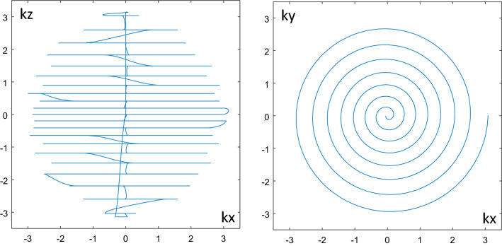
Objective: This review article gives an account of the development of the MR-encephalography (MREG) method, which started as a mere 'Gedankenexperiment' in 2005 and gradually developed into a method for ultrafast measurement of physiological activities in the brain. After going through different approaches covering k-space with radial, rosette, and concentric shell trajectories we have settled on a stack-of-spiral trajectory, which allows full brain coverage with (nominal) 3 mm isotropic resolution in 100 ms. The very high acceleration factor is facilitated by the near-isotropic k-space coverage, which allows high acceleration in all three spatial dimensions.

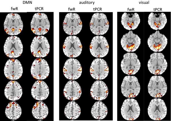
Methods: The methodological section covers the basic sequence design as well as recent advances in image reconstruction including the targeted reconstruction, which allows real-time feedback applications, and-most recently-the time-domain principal component reconstruction (tPCR), which applies a principal component analysis of the acquired time domain data as a sparsifying transformation to improve reconstruction speed as well as quality.

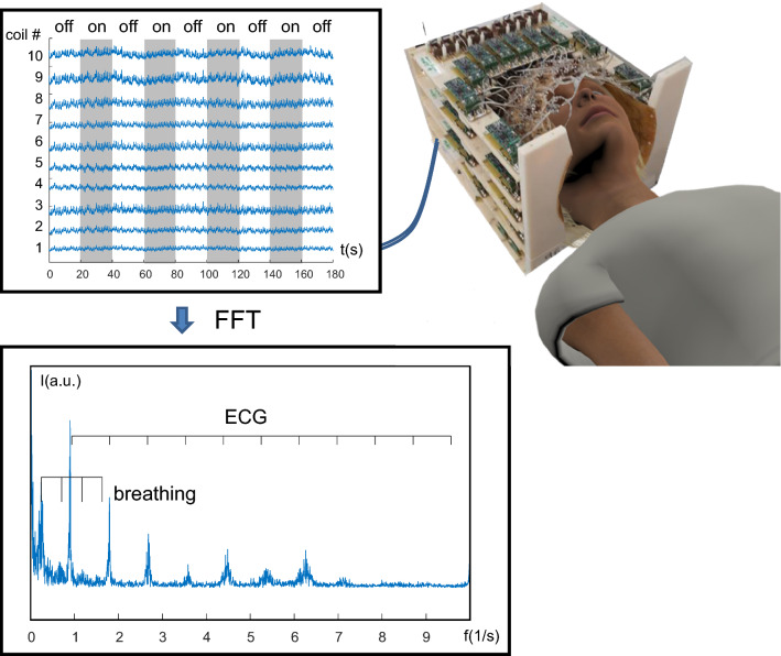
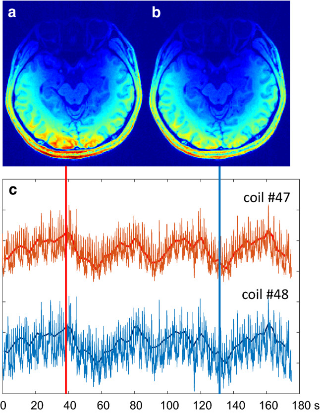
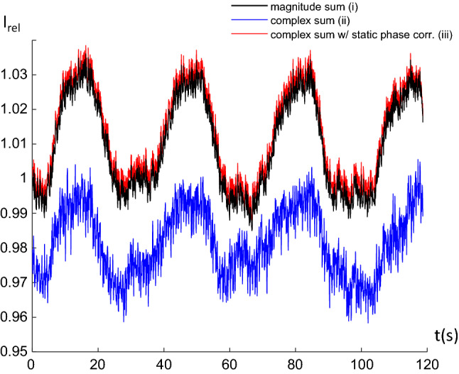
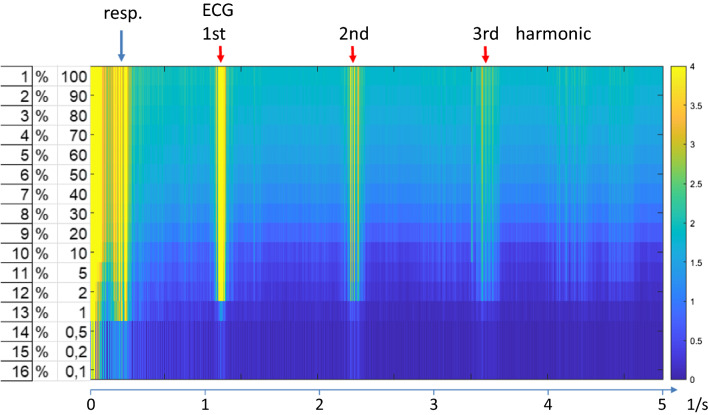
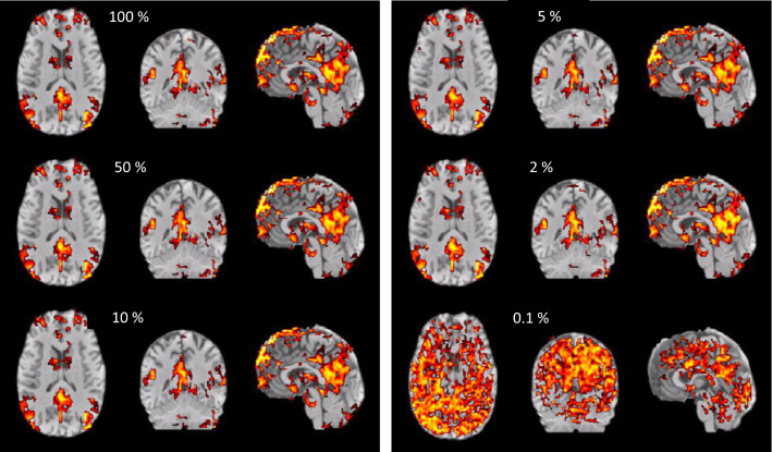
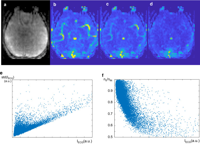
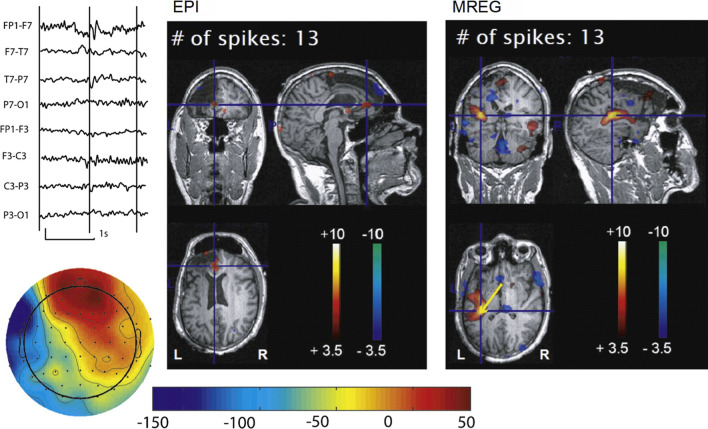
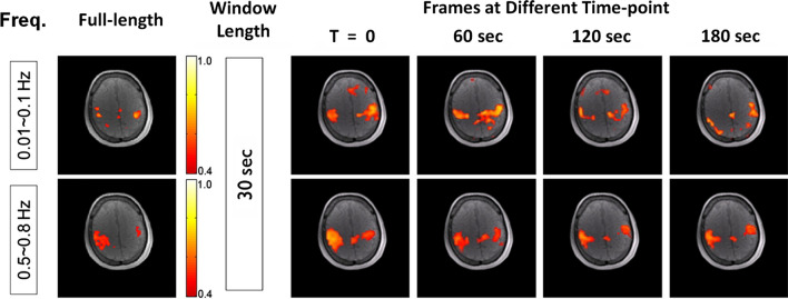
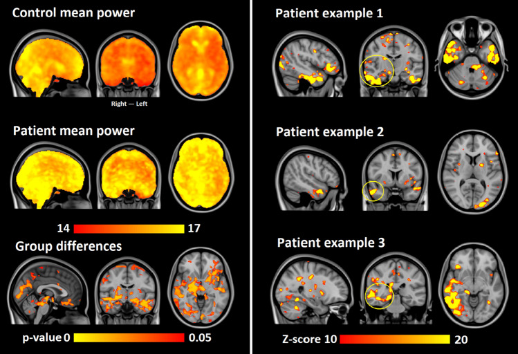
Applications: Although the BOLD-response is rather slow, the high speed acquisition of MREG allows separation of BOLD-effects from cardiac and breathing related pulsatility. The increased sensitivity enables direct detection of the dynamic variability of resting state networks as well as localization of single interictal events in epilepsy patients. A separate and highly intriguing application is aimed at the investigation of the glymphatic system by assessment of the spatiotemporal patterns of cardiac and breathing related pulsatility.

Discussion: MREG has been developed to push the speed limits of fMRI. Compared to multiband-EPI this allows considerably faster acquisition at the cost of reduced image quality and spatial resolution.

Keywords: Functional magnetic resonance imaging; Magnetic resonance imaging.

Fig. 1

Basic principle of OVOC-experiment. The signal of each coil is separately measured and recorded and can be displayed as multi-channel signal display just as in EEG (top left). Fourier transformation of the signal time course reveals distinct peaks attributed to breathing and ECG-related signal pulsatility. Due to its very ‘spiky’ nature, especially ECG shows pronounced intensity at higher harmonics. Only the spectrum from channel 10 is shown

Fig. 2

Relative signal intensity I_stof the spectral peak at the stimulus frequency compared to baseline in a visual stimulation experiment in the individual coil elements of the 64-channel coils used. Sample images of coils with high intensity show that the respective coil elements cover the visual cortex. The relative change is rather small, since the activated voxels represent just a small fraction of the total signal in each coil

Fig. 3

Activation ‘images’ at the top of the BOLD response (a) and during rest (b). Images are generated by sum-of-squares combination of reference images of all individual coil elements weighted with the actual signal intensity in each coil element. c shows individual signal time courses in two coils. Signals have been low pass filtered to reduce ECG-dependent flickering (solid lines in c). a Corresponds to the time indicated by the red vertical line in c, b to the time indicated by the blue vertical line

Fig. 4

Sampling schemes of COBRA (a) compared to VIPR (b) and HYPR (c). The lines under the trajectories indicate the reconstruction strategy: COBRA uses repetitive sampling of identical radial spokes with reconstruction of each individual timeframe to preserve the temporal fidelity of the scan, VIPR is based on a sophisticated view sharing scheme with a trade-off between temporal and spatial resolution (colored lines indicate combinations of data used for reconstruction of individual time frames), whereas HYPR generates images with high temporal resolution by weighting the final high-resolution image with the low-resolution image of individual time frames. Note that in all sampling schemes acquisition runs continuously, the collection into packages of 4 spokes is for visualization only. The dotted lines in the top left diagram in a illustrate how multiple radial spokes are converted into a single shot rosette trajectory

Fig. 5

a Field map and (b) map of susceptibility induced field gradient over the brain. c Shows the histogram of the pixel count as a function of the field gradient clearly demonstrating the dominance of susceptibility effects in the z-direction

Fig. 6

Color-coded image display of four consecutive activation periods of visual stimulation with a flickering checkerboard (20 s on–20 s off). Each frame shows normalized signal amplitudes in activated voxels (thresholded at t values > 30). The number in each frame represents the mean and standard deviation of the BOLD arrival time over the activated signal time courses. The BOLD arrival time is measured as the time at which the signal reaches half its maximum in each stimulation period. The yellow bar at the bottom indicates the stimulus-on period, which starts 1 s into each frame (vertical red lines). The BOLD arrival time map representing the mean arrival time over 4 stimulation periods is shown on top right, the color bar represents the BOLD arrival time in seconds. At bottom right three signal time courses at different BOLD arrival times are displayed. Numbers in each frame represent the mean BOLD arrival time and standard deviation for each stimulation period. The mean arrival time over all 4 periods is 5.99 ± 1.25 s

Fig. 7

Projections of the actual k-space trajectory onto the kx-kz-resp. kx-ky-plane

Fig. 8

Signal time course over the visual cortex generated as the sum of the magnitude signals of a fully reconstructed dataset (black) compared to the complex sum reconstructed with targeted reconstruction without (blue) and with (red) correction for static phase (same data as in Fig. 5 in ref. [43] were used). Reference signal and complex sum with phase correction are nearly identical, the red line has been slightly shifted in the plot for clarity

Fig. 9

Comparison of ICA-based RSN-analysis for frame-wise reconstruction (fwR) with temporal principle component reconstruction (tPCR). Detected default mode network (DMN), auditory, and primary visual networks are virtually identical for both reconstruction modes

Fig. 10

Image representation of frequency spectra of signal timecourse as a function of the percentage of PCA-components used in the final reconstruction. The horizontal axis represents frequency, the vertical axis represents the percentage of PCA-components used in the final recombination of the PCA-components. Signal intensities are scaled in arbitrary units, the yellow bands represent physiological signals as indicated at the top

Fig. 11

ICA reconstruction of the default mode network using a different percentage of the PCA components. In the example shown even 2% of the components deliver nearly identical networks compared to full reconstruction. Only at 0.1% network reconstruction breaks down

Fig. 12

a Maximum intensity projection (MIP) through a 4.8 cam thick slab at the height of the visual cortex, (b) corresponding MIP of the pixel-wise temporal noise measured as the standard deviation of the signal timecourse after linear detrending. c MIP of the pixelwise temporal noise after filtering out the ECG-peak at 1.2 ± 0.1 Hz from the frequency spectrum. d MIP of the temporal noise after low pass filtering with a cutoff frequency of 1 Hz. e Plot of the signal intensity of the frequency peak at the ECG-frequency against temporal noise shows a clear correlation e. f Reduction of temporal noise after filtering out the ECG. Peak alone (corresponding to c)

Fig. 13

BOLD activation maps associated with left frontal epileptic spikes in a patient with focal cortical dysplasia with a previous frontal resection that did not result in seizure freedom. While the EPI map shows a small activation near the resection border, the MREG map reveals a much larger activated area extending into parietal regions. In the left upper corner a typical epileptic spikes is visible in the EEG trace over the left fronto-temporal area as well as a voltage map derived from this spike. (Fig. 5 from Jacobs et al. [52]) adapted from

Fig. 14

Resting-state connectivity in the primary motor cortex in the 0.01–0.1 Hz (top row) and 0.5–0.8 Hz (bottom row) frequency bands. While the connectivity calculated over the full-length scan (left column) involves the same motor areas in both frequency bands, the connectivity calculated over 30-s time windows (right columns) is highly variable in the 0.01–0.1 Hz band, also involving spurious regions outside motor areas. The calculated sliding-window connectivity is much more reliable in the 0.5–0.8 Hz band (adapted from Fig. 4 from Lee et al. [67])

Fig. 15

Common resting-state networks extracted by ICA from EPI (top) and MREG (bottom) data using various time window lengths (shown in the multiple columns). Images with a red background denote that a component corresponding to the given network could not be found. For time window longer than 300 s, all networks could be successfully detected with both sequences. However, for shorter time windows, the detection is only reliable when using MREG data. (adapted from Figs.  7, 8 from Akin et al. [69])

Fig. 16

Example of human full band MREG signal with FFT power spectrum presenting three main physiological pulsations in the spectrum peaks. MREG signal was further band passed for quantification and mapping into anatomy. The VLF band and representative signal in orange, respiratory pulsations in green and cardiac pulsations in red, respectively, overlaid over MNI 152 space. Please also notice the harmonic power spectrum peaks over the full 5 Hz power spectrum highlighting the precision of the MREG signal

Fig. 17

Example of optical flow analysis of MREG cardiac pulse propagation over the brain from the Alzheimer brain analysis revealing momentary pulsation abnormality occurring during the cardiac impulse arrival in the brain. The abnormality is highly variable over time and space and affects the BOLD signal variance significantly, see also [81]. Due to critical 10 Hz sampling rate of the MREG, the abnormality can be quantified with unprecedented spatiotemporal precision. To see how the cardiac impulse propagates over the brain in video, please see also: https://www.newscientist.com/article/mg23130864-200-best-look-yet-at-how-our-brains-sewage-system-flushes-out-waste/

Fig. 18

The respiratory pulsation power is altered significantly in epilepsy. Top: the mean of control and patient respiratory brain pulsation power. Bottom: the significant pulsation power changes (p < 0.05 FSL randomize TFCE-corrected for voxel-level). Right panel: patient examples showing individual patient’s increase > 10 standard deviations above control (n = 100) respiratory pulsation power

Fig. 19

a Result from 1-shot, 2-shot, and 3-shot segmented MREG acquired with TR of 96, 180, and 264 ms, respectively, shows improvement in image quality of segmented acquisition. b Comparison of seed-based RSN for 1-shot (top) and 3-shot (bottom) trajectories shows nearly identical results

Fig. 20

Comparison of activation maps acquired with spin-echo MREG (TR = 250 ms) (top left) and SMS-EPI (TR = 1300 ms) (top right) for checkerboard stimulation. Activation maps are overlaid to a single time frame of the measurement series. Both datasets had identical spatial resolution (3 × 3 × 3 mm³), stimulus was presented in a block paradigm with interval times 18 s on–18 s off. Color bars represent t values with the t threshold indicated by the horizontal green bar. The t threshold has been determined by the method of surrogate data [139] to account for the different number of data points as well as the different noise properties dependent on the temporal resolution. The bottom graph shows the signal time course in the activated areas, it also includes result from a standard EPI experiment

References

1. Hennig J, Zhong K, Speck O. MR-encephalography: fast multi-channel monitoring of brain physiology with magnetic resonance. Neuroimage. 2007;34:212–219. - PubMed
1. Mistretta CA, Wieben O, Velikina J, Block W, Perry J, Wu Y, Johnson K, Wu Y. Highly constrained backprojection for time-resolved MRI. Magn Reson Med. 2006;55:30–40. - PMC - PubMed
1. Hennig J, Welz AM, Schultz G, Korvink J, Liu Z, Speck O, Zaitsev M. Parallel imaging in non-bijective, curvilinear magnetic field gradients: a concept study. Magn Reson Mater Phys Biol Med. 2008;21:5–14. - PMC - PubMed
1. Littin S, Jia F, Layton KJ, Kroboth S, Yu H, Hennig J, Zaitsev M. Development and implementation of an 84-channel matrix gradient coil. Magn Reson Med. 2018;79:1181–1191. - PubMed
1. Kroboth S, Layton KJ, Jia F, Littin S, Yu H, Hennig J, Zaitsev M. Optimization of coil element configurations for a matrix gradient coil. IEEE Trans Med Imaging. 2017 doi: 10.1109/TMI.2017.2743463. - DOI - PubMed
LinkOut - more resources