Early Emergence of Solid Shape Coding in Natural and Deep Network Vision

Abstract

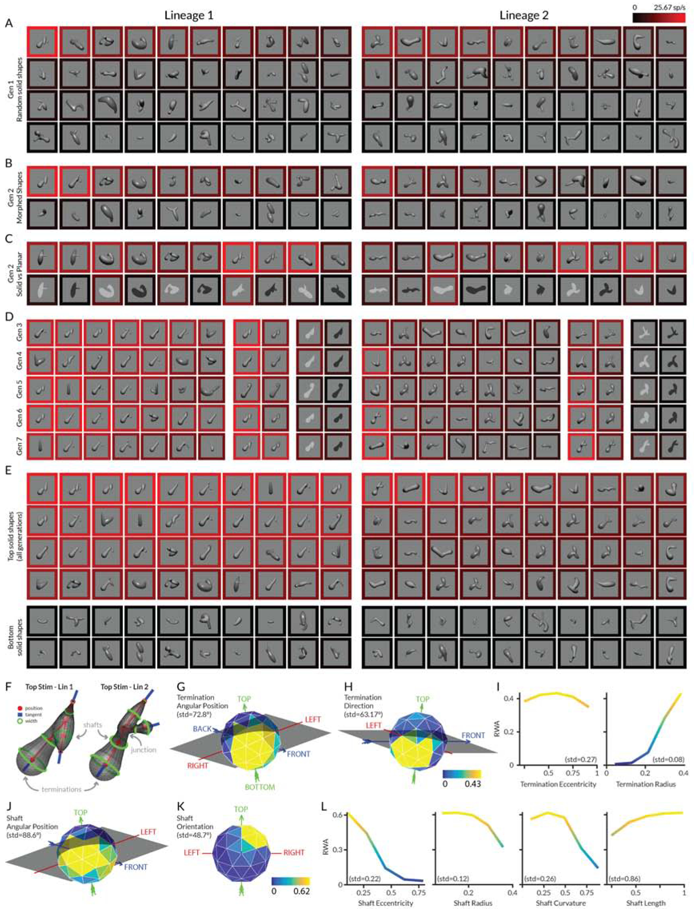
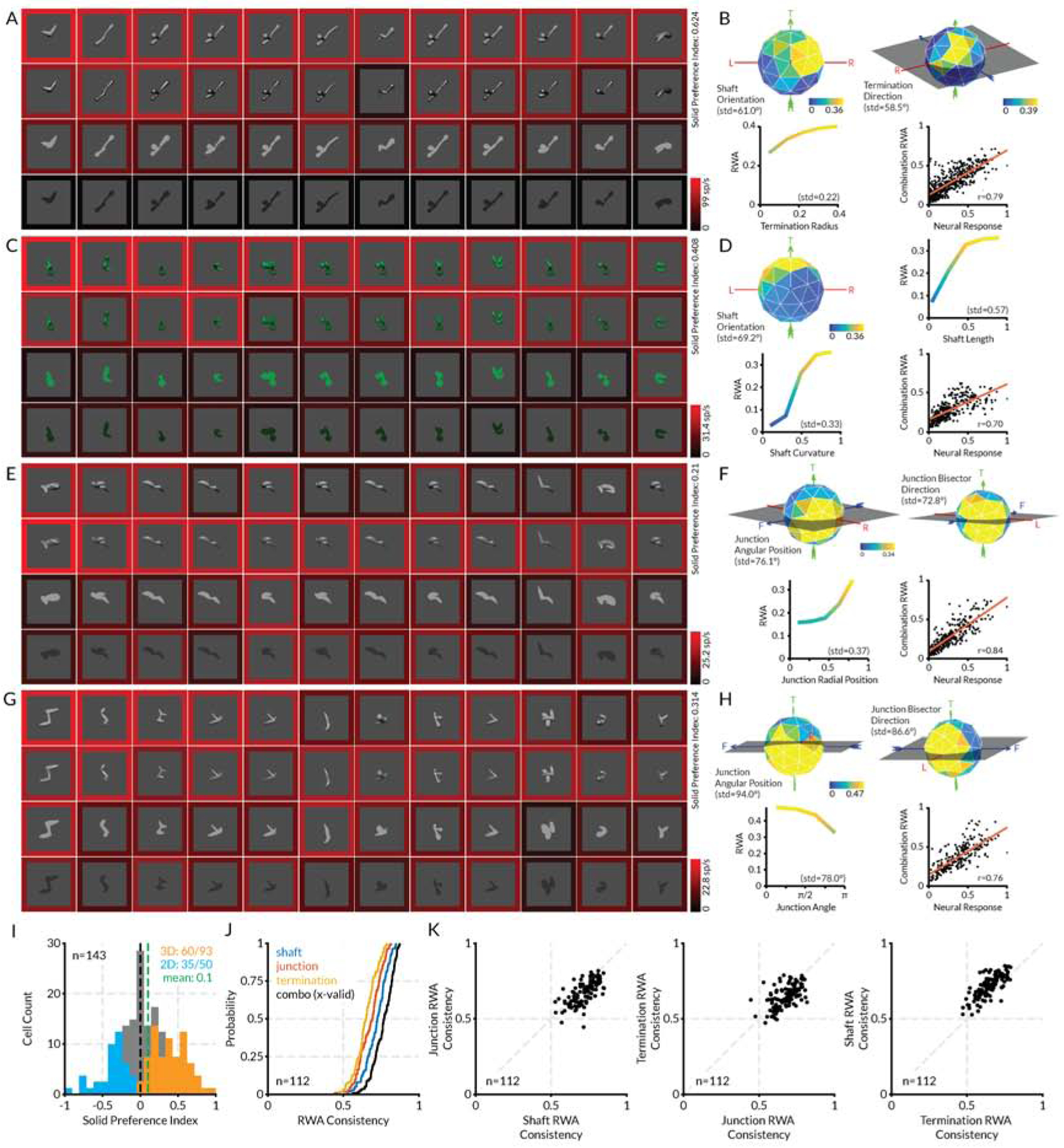
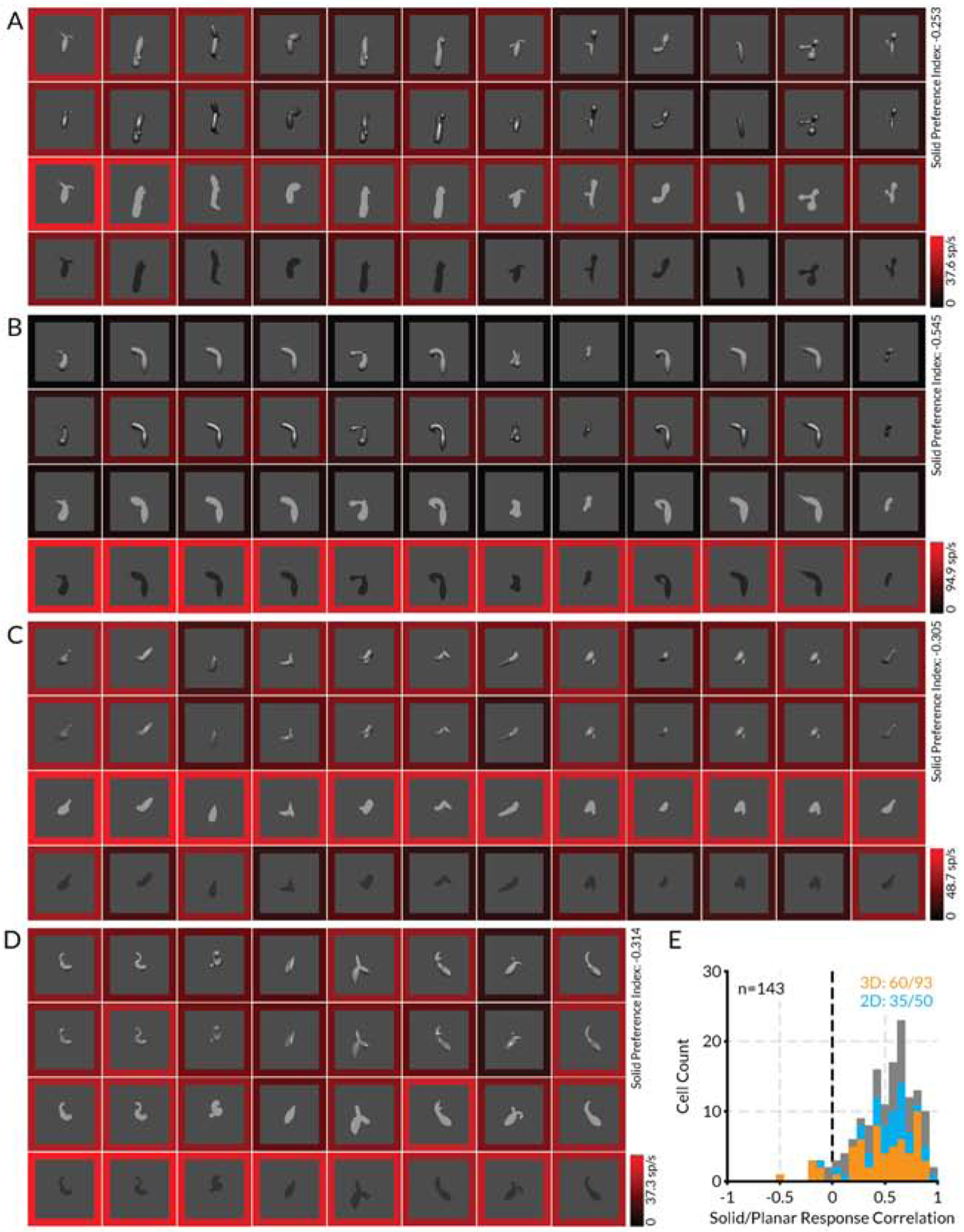
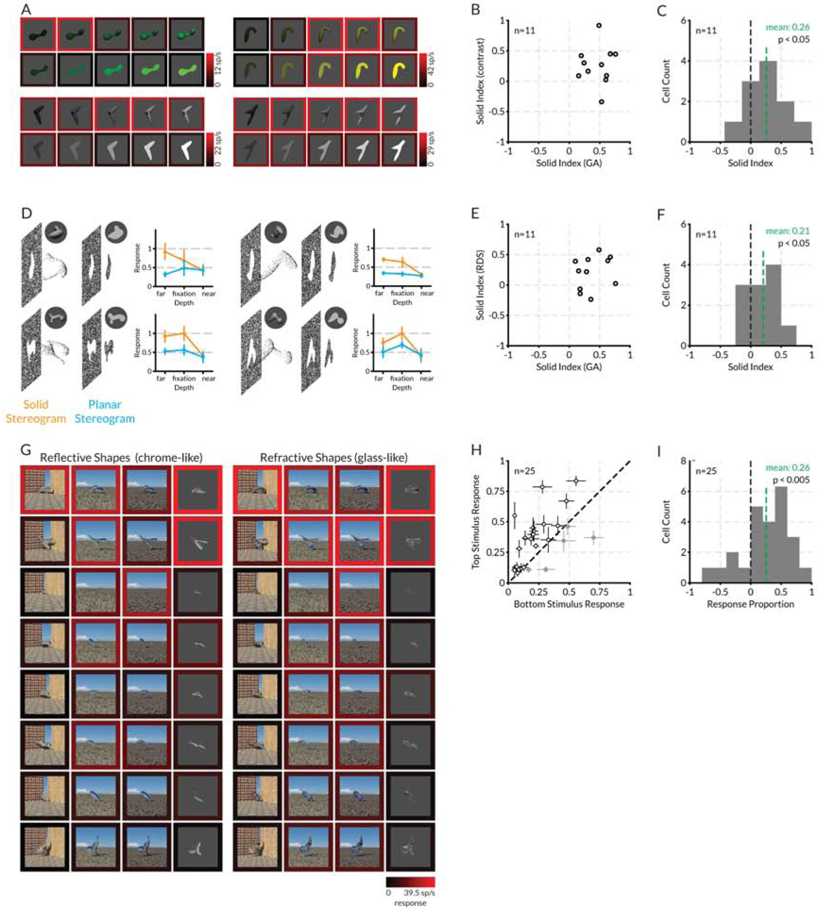
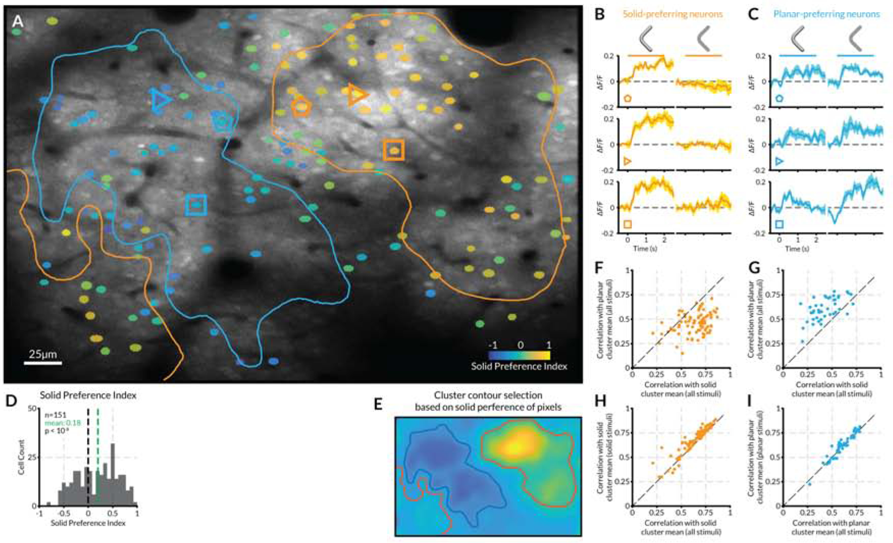
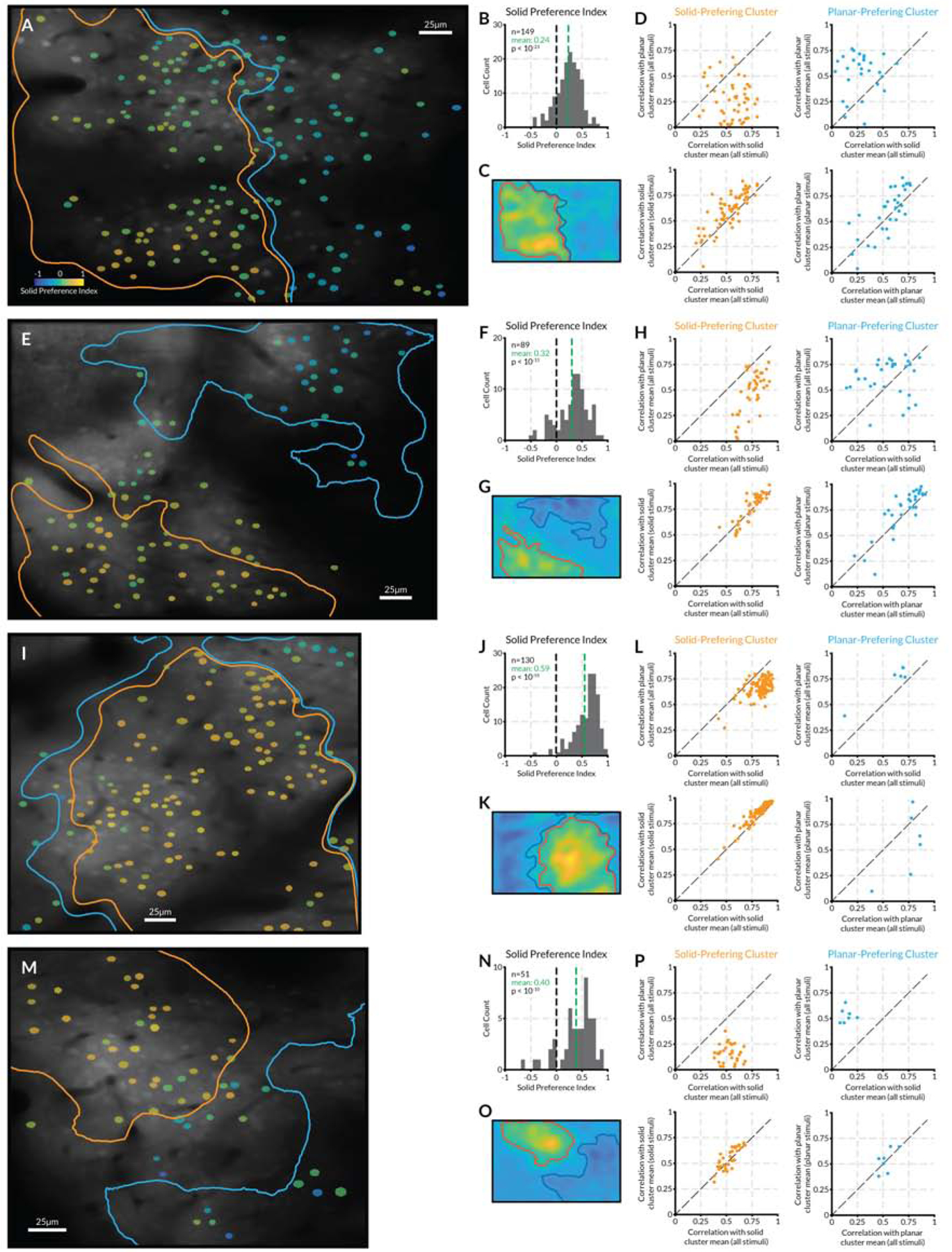
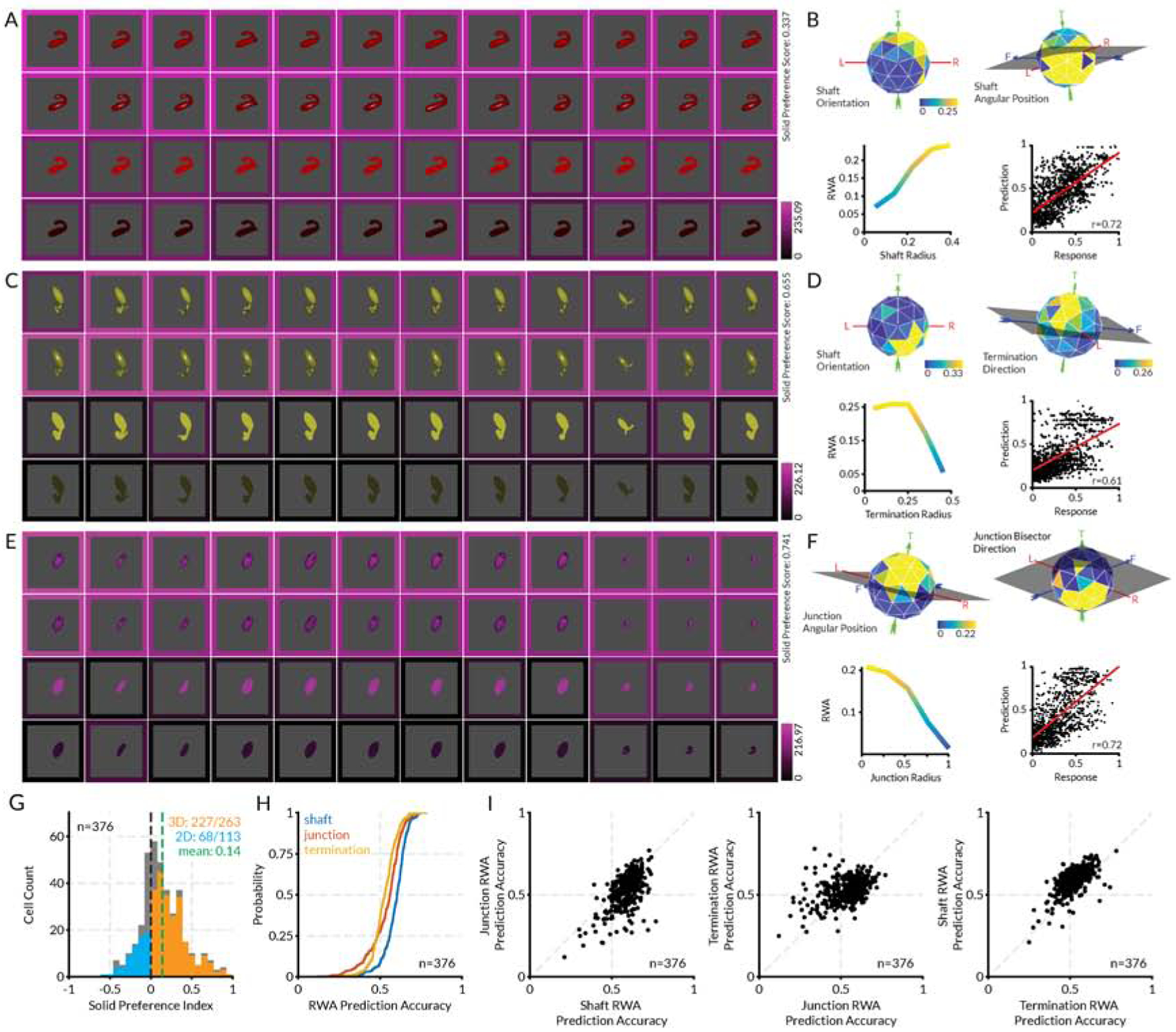
Area V4 is the first object-specific processing stage in the ventral visual pathway, just as area MT is the first motion-specific processing stage in the dorsal pathway. For almost 50 years, coding of object shape in V4 has been studied and conceived in terms of flat pattern processing, given its early position in the transformation of 2D visual images. Here, however, in awake monkey recording experiments, we found that roughly half of V4 neurons are more tuned and responsive to solid, 3D shape-in-depth, as conveyed by shading, specularity, reflection, refraction, or disparity cues in images. Using 2-photon functional microscopy, we found that flat- and solid-preferring neurons were segregated into separate modules across the surface of area V4. These findings should impact early shape-processing theories and models, which have focused on 2D pattern processing. In fact, our analyses of early object processing in AlexNet, a standard visual deep network, revealed a similar distribution of sensitivities to flat and solid shape in layer 3. Early processing of solid shape, in parallel with flat shape, could represent a computational advantage discovered by both primate brain evolution and deep-network training.

Keywords: 3D; V4; cortex; deep network; neural coding; object; primate; shape; ventral pathway; vision.

Figure 1.. Area V4 encodes solid shape information—introductory example.

(A) First generation (Gen 1) of 40 random stimuli per lineage. Each stimulus was rendered with a lighting model based on either a matte or polished surface illuminated by an infinite distance point source from the viewer’s direction. Stimuli were centered on and sized to fit within the previously mapped receptive field of an individual V4 neuron and flashed in random order for 750 ms each (interleaved with 250 ms blank periods), against a uniform gray background, while the monkey performed a fixation task. The response rate for each stimulus was calculated as the average number of spikes/s across the 750 ms presentation periods and across 5 repetitions of each stimulus. The neuron’s average response to each stimulus is represented by the color of the surrounding border, referenced to the scale at the upper right, with bright red corresponding to 26 spikes/s. Stimuli in each block are ordered by descending response strength from the upper left to the lower right. (B) Half of Gen 2 comprised partially morphed descendants of ancestor stimuli from Gen 1 plus additional random stimuli. (C) The other half of Gen 2 comprised tests of high response Gen 1 stimuli rendered as solid vs. flat shapes. (D) Highest response stimuli and example solid/flat comparisons in Gen 3–7. (E) Highest and lowest response stimuli across all generations. (F) Parameterization of shaft, junction, and termination shape. (G–L) Response weighted average (RWA) analysis of response strength. Each panel shows average normalized response strength as a function of geometric dimensions used to describe shaft or termination shape. Each plot represents a slice through the RWA at the location of the overall RWA peak across all dimensions (rather than a collapsed average across the other dimensions). Spherical (object-centered position and termination direction) and hemispherical dimensions (shaft orientation) are shown as spherical polygons, in some cases tilted and rotated to reveal the tuning peak. The arrows and labels (LEFT, RIGHT, TOP, BOTTOM, BACK, FRONT) indicate the original directions in the stimulus from the monkey’s point of view. Normalized response strength is indexed to a color scale for shafts (below K) and a color scale for terminations (below H). Color is a redundant cue for response strength in the Cartesian plots. See also Figure S1.

Figure 2.. Area V4 encodes solid shape information—additional examples.

(A) Highest response stimuli (columns) for the first example neuron, tested in four rendering conditions (rows). Scale bar at bottom right indexes the border color representation of average neural response to each stimulus. (B) Plots of RWA strength for this neuron, selected to highlight dimensions with strongest tuning, plus a scatterplot of RWA responses vs. observed responses. (C–H) Plots for the three other example neurons. Details as in (a) and (b). (I) Histogram distribution of solid shape preference index (SP). Values significantly greater or less than 0 (t-test, two-tailed, p < 0.05) are plotted in orange and blue, respectively. (J) Cumulative distributions of RWA/observed correlations for shaft, junction, and termination RWAs. (K) Comparisons of prediction accuracies for shaft, junction, and termination RWAs. See also Figure S2.

Figure 3.. Area V4 encodes flat shape information—example.

(A–D) Highest response stimuli (columns) for four example neurons, tested in four rendering conditions (rows), showing stronger responses to flat shapes. Scale bar at bottom right of each plot indexes the border color representation of average neural response to each stimulus. (E) Distribution of correlation values between highest response solid rendering condition (either shading or specular) and highest response flat rendering condition (either bright or dark) across all stimuli tested in the four rendering conditions.

Figure 4.. V4 solid shape coding generalizes across different image cues.

(A) Comparison of solid and flat stimulus responses across a range of figure/background contrasts, for four example solid-preferring V4 neurons. In each case, responses to solid stimuli, within an optimum contrast range, were stronger, as shown by the brighter red surrounds (indexed to the color scale bars on the bottom right of each plot). (B) Scatterplot of solid preference values for 11 neurons with significantly positive solid preference values in the genetic algorithm dataset (randomization t-test, two-tailed, p < 0,05), tested across contrasts as in (A). (C) Histogram of solid preference values for the same 11 neurons. The mean solid preference value for these neurons in the genetic algorithm was 0.46 and this was significantly greater than 0 (t-test, two- tailed, p <0.001). The mean solid preference value in the contrast test, based on averaging responses across the full contrast ranges, was 0.26 and this was significantly greater than 0 (t-test, two-tailed, p < 0.05). (D) Diagrams and normalized response plots for four example V4 neurons, comparing responses to solid vs. planar random dot stereogram versions of high response stimuli from the genetic algorithm experiment, presented at three stereoscopic depths relative to the fixation plane. Bars indicate standard error of the mean across 5 repetitions. (E) Scatterplot of solid preference values for 11 neurons with significantly positive solid preference values in the genetic algorithm dataset (randomization t-test, two-tailed, p < 0,05), tested with solid and planar stereograms as in (D). (F) Histogram of solid preference values for the same 11 neurons. The mean solid preference value for these neurons in the genetic algorithm was 0.37 and this was significantly greater than 0 (t-test, two-tailed, p <0.001). The mean solid preference value in the random dot stereogram test, based on averaging responses across depths, was 0.21 and this was significantly greater than 0 (t-test, two-tailed, p < 0.05). (G) Responses of a single example solid-preferring V4 neuron to 8 stimuli (rows, in descending order of response strength in the original genetic algorithm dataset) in four chrome-like renderings and four glass-like renderings (columns). Response levels are indicated by border color, indexed to the scale bar at lower right. (H) Scatterplot of average responses of 25 neurons tested in the same way, to the top vs. bottom genetic algorithm stimuli, averaged across the refraction and reflection rendering conditions (e.g., the top and bottom rows in (C)). (I) Histogram of response proportion index values for the same 25 neurons. The RP mean across the 25 neurons was 0.26 and this was significantly greater than 0 (t-test, two-tailed, p < 0.005). See also Figure S3.

Figure 5.. Area V4 micro-organization includes flat and solid shape modules—introductory example.

(A) Anatomical average image of a section of V4 cortical surface (anatomical scale bar at lower left). Neurons with significant (based on multiple tests; see STAR Methods) fluorescent responses to stimuli (Figure S4) are overlaid with a color indexing their preference for flat (blue) or solid (yellow) stimuli (SP; see solid preference scale bar at lower right). (B) Peri-stimulus time fluorescence plots for example solid-preferring neurons indicated by orange polygons in (A). Horizontal bars span the 2 s stimulus presentation period for solid (left) and flat (right) stimuli. (C) Example flat-preferring neurons; details as in (B). (D) Distribution of solid preference values for neurons in this region. The mean solid preference value of 0.18 is significantly greater than 0 (t-test, two-tailed, p < 10⁻⁶). (E) Smoothed map of pixels solid preference values in this imaging region, used as the basis for drawing cluster boundaries (see STAR Methods) shown in (A). (F) Correlations of stimulus response patterns for neurons in the upper right solid cluster (orange contour in (A)) with the average response pattern in that solid cluster (horizontal axis) vs. the average response pattern in the planar cluster (blue contour in (A)). (G) Correlations of stimulus response patterns for neurons the planar cluster (blue contour in (A)) with solid and planar cluster averages. (H) Correlations of solid cluster neurons with solid cluster average across all stimuli (horizontal axis) vs. solid stimuli only (vertical axis). (I) Correlations of planar cluster neurons with planar cluster average across all stimuli (horizontal axis) vs. planar stimuli only (vertical axis).

Figure 6.. Area V4 micro-organization includes flat and solid shape modules—additional examples.

(A–D, E–H, I–L) Three imaging regions studied with flashing stimuli (Figure S4), as in Figure 5. Details as in Figure 5. (M–P) Imaging region studied with drifting stimuli (Figure S5). These data leave open questions about distribution of cluster sizes across larger surface regions, relationship of clusters to organization for other tuning dimensions in V4, and depth profiles of clusters, which would require electrophysiology to measure.

Figure 7.. AlexNet layer 3 neurons exhibit similar flat and solid shape tuning.

(A) Highest response stimuli (columns) for an example layer 3 neuron, tested in four rendering conditions (shading, shading + specularity, bright flat, dark flat, rows). (B) RWA plots for this unit, selected to highlight dimensions with strongest tuning, plus a scatterplot of RWA values vs. observed activations. (C–F) Two additional example layer 3 neurons. Details as in (A) and (B). (G) Distribution of solid preference values for 376 unique layer 3 neurons. The mean value of 0.15 was significantly greater than 0 (t-test, two-tailed, p < 10⁻²¹). (H) Cumulative distributions of correlations between observed activations by genetic algorithm stimuli and values in RWAs based on the geometry of shafts, junctions, and terminations. (I) Scatterplots comparing correlations with observed activations and RWAs based on shafts, junctions, and termination. See also Figure S6.

References

1. Koenderink JJ (1984). What does the occluding contour tell us about solid shape? Perception 13, 321–330. - PubMed
1. Richards WA, Dawson B, and WhittingDton D (1986). Encoding contour shape by curvature extrema. J. Opt. Soc. Amer. A 3, 1483–1491. - PubMed
1. Richards WA, Koenderink JJ, and Hoffman DD (1987). Inferring three-dimensional shapes from two-dimensional silhouettes. J. Opt. Soc. Amer. A 4, 1168–1175.
1. Beusmans JMH, Hoffman DD, and Bennett BM (1987). Description of solid shape and its inference from occluding contours. J. Opt. Soc. Amer. A 4, 1155–1167.
1. Tse PU (2002). A contour propagation approach to surface filling-in and volume formation. Psych. Rev 109, 91–115. - PubMed
Publication types
LinkOut - more resources