Optical-Clock-Based Time Scale

Abstract

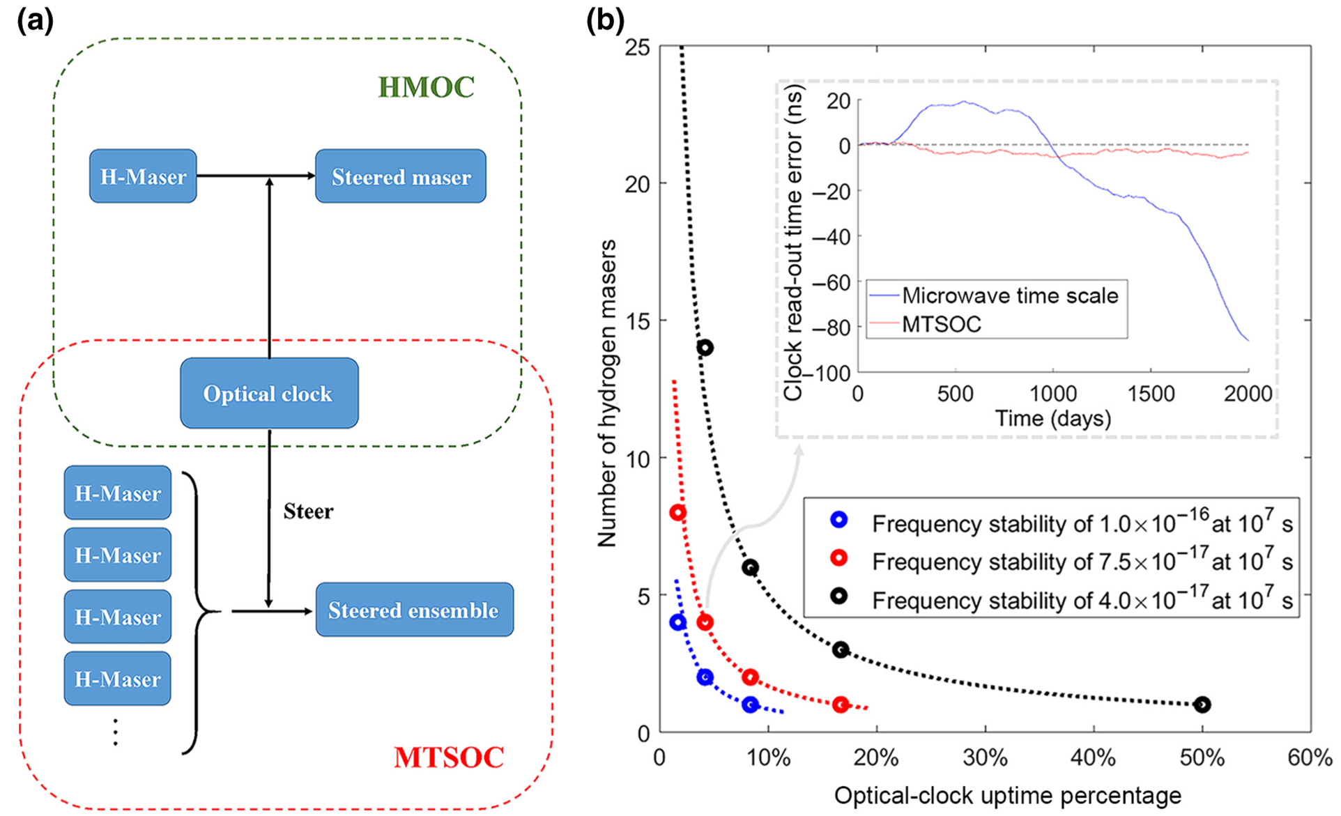
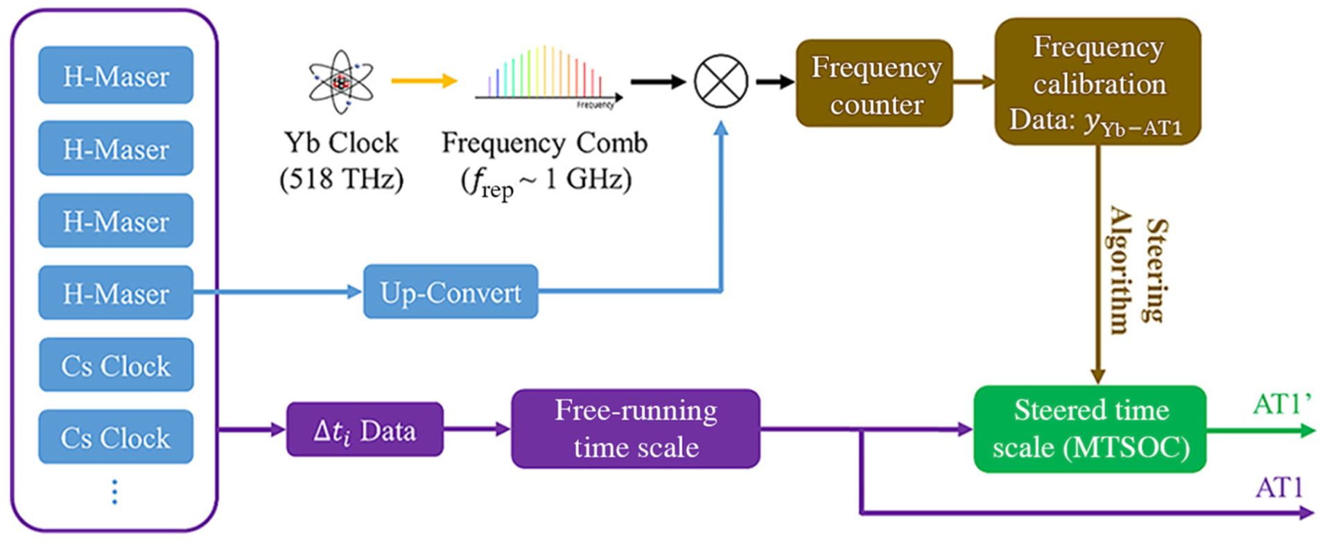
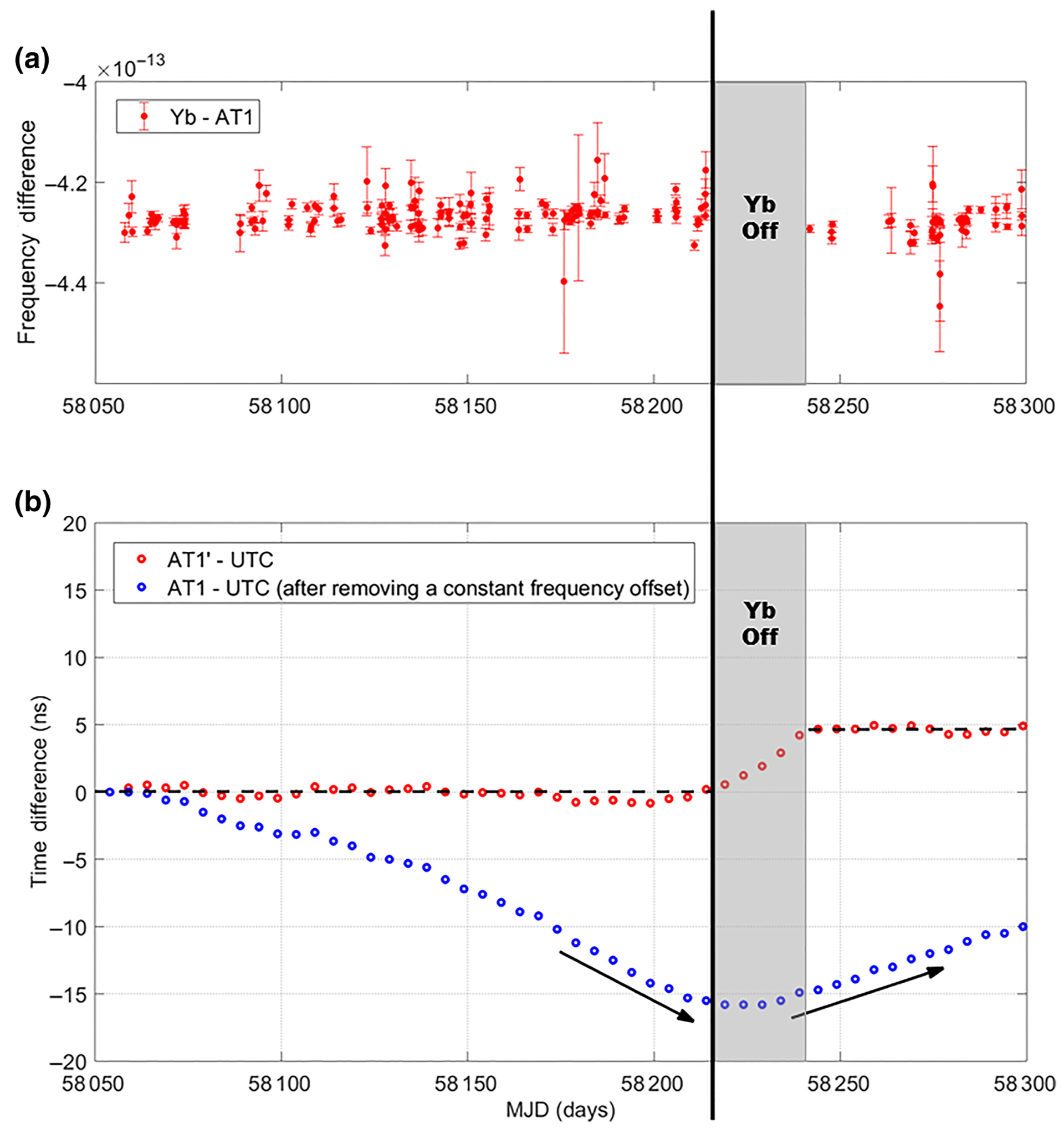
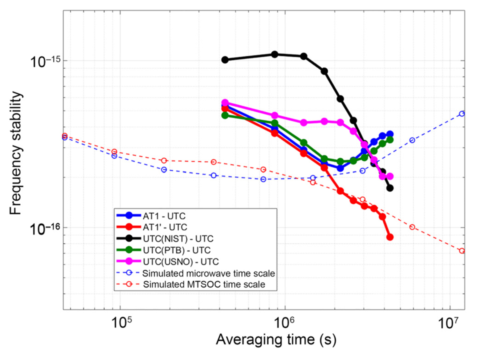
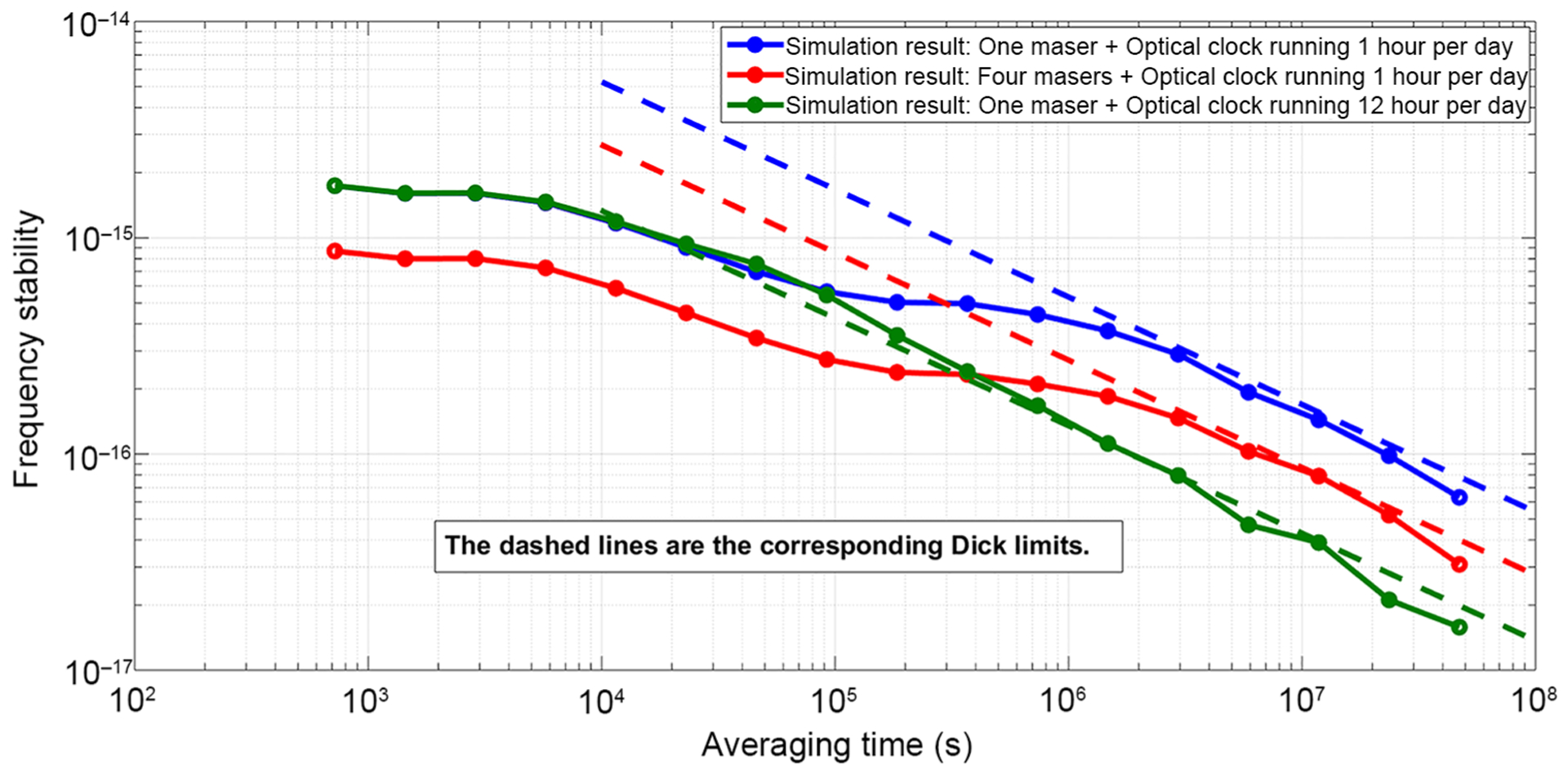
A time scale is a procedure for accurately and continuously marking the passage of time. It is exemplified by Coordinated Universal Time (UTC) and provides the backbone for critical navigation tools such as the Global Positioning System. Present time scales employ microwave atomic clocks, whose attributes can be combined and averaged in a manner such that the composite is more stable, accurate, and reliable than the output of any individual clock. Over the past decade, clocks operating at optical frequencies have been introduced that are orders of magnitude more stable than any microwave clock. However, in spite of their great potential, these optical clocks cannot be operated continuously, which makes their use in a time scale problematic. We report the development of a hybrid microwave-optical time scale, which only requires the optical clock to run intermittently while relying upon the ensemble of microwave clocks to serve as the flywheel oscillator. The benefit of using a clock ensemble as the flywheel oscillator instead of a single clock can be understood by the Dick-effect limit. This time scale demonstrates for the first time subnanosecond accuracy over a few months, attaining a fractional frequency stability of 1.45 × 10^-16 at 30 days and reaching the 10^-17 decade at 50 days, with respect to UTC. This time scale significantly improves the accuracy in timekeeping and could change the existing time-scale architectures.

FIG. 1.

Concept of an optical-clock-based time scale. (a) Illustrates the HMOC architecture (green dashed box) and the MTSOC architecture (red dashed box). (b) Summarizes the relation between the number of masers and the optical-clock uptime for different performance goals (blue, 1.0 × 10⁻¹⁶ at 10⁷ s; red, 7.5 × 10⁻¹⁷ at 10⁷ s; black, 4.0 × 10⁻¹⁷ at 10⁷ s), when an optical clock runs once a day. The dots are the results of simulations, and the dashed curves are hyperbolas, which well fit the dots. The inserted plot of (b) shows an example of the simulation in time series. The blue solid curve is the read-out time error of a microwave time scale composed of four hydrogen masers, and the red solid curve is the read-out time error of a MTSOC composed of the four hydrogen masers and an optical clock of 4.2% uptime. Note (b) is plotted based on the simulations in [24].

FIG. 2.

Experimental scheme of optical-clock-based time scale AT1′ and comparison to free-running time scale AT1.

FIG. 3.

(a) Shows the fractional frequency difference between the Yb clock and AT1 during MJD 58054–58214. Note AT1, composed of a few hydrogen masers and a few commercial cesium clocks, is a free-running microwave time scale at NIST. (b) Shows the time difference between AT1′ and UTC (red dots) during MJD 58054–58214. AT1′ is the NIST time scale that is steered to the Yb clock. AT1′ is set to 0 ns initially. AT1′ has a root-mean-square variation of 0.4 ns with respect to UTC during MJD 58054–58214. The time difference between AT1 and UTC (blue dots) is shown for reference. A constant frequency offset of +4.278 × 10⁻¹³ (measured from the first two points on the plot) in AT1 has already been removed. (c),(d) Show the behavior of AT1′ and AT1 during MJD 58215–58300. During MJD 58215–58240 (gray region), the Yb clock ceases regular operation. After Yb-clock data resumes on MJD 58241, AT1′ becomes flat with respect to UTC [black dashed line in (d)] indicating prompt frequency recalibration. The frequency change of AT1 is illustrated by the black arrows.

FIG. 4.

Frequency stability of AT1, AT1′, UTC(NIST), UTC(PTB), and UTC(USNO), for MJD 58054–58214. The frequency stability is characterized by modified total deviation, and error bars (omitted here for plot clarity) are provided in Appendix C. The dashed curves show the simulation result. Note, the simulated MTSOC time scale (red dashed curve) is composed of the simulated microwave time scale (blue dashed curve) and a simulated optical clock that runs one hour per day.

FIG. 5.

Comparison between the Dick limits (dashed lines) and simulation results in [24].

References

1. Getting IA, Perspective/navigation – the Global Positioning System, IEEE Spectrum 30, 36 (1993).
1. Bregni S, Synchronization of Digital Telecommunications Networks (John Wiley & Sons, 2002).
1. Fang X, Misra S, Xue G, and Yang D, Smart grid – the new and improved power grid: a survey, IEEE Commun. Surv. Tutor 14, 944 (2011).
1. Lombardi MA, Novick AN, Neville-Neil G, and Cooke B, Accurate, traceable, verifiable time synchronization for world financial markets, J. Res. Natl. Inst. Stand. Technol 121, 436 (2016). - PMC - PubMed
1. Riehle F, Optical clock networks, Nat. Photonics 11, 25 (2017).
LinkOut - more resources