Comparison of distributed memory algorithms for X-ray wave propagation in inhomogeneous media

Abstract

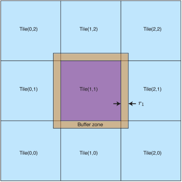
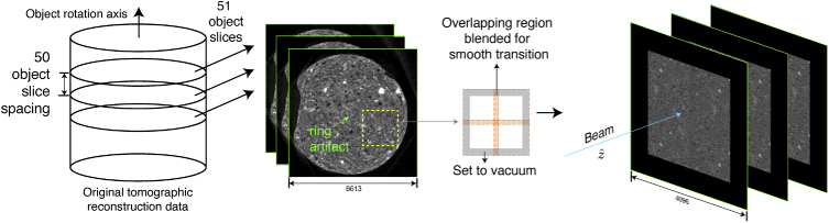
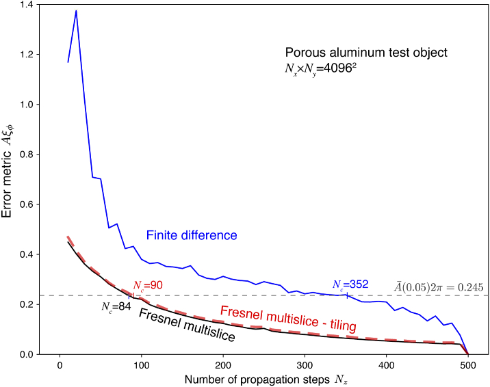
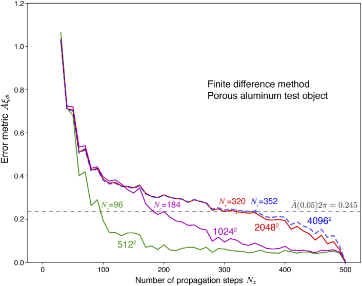
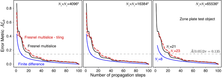
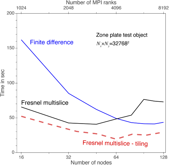
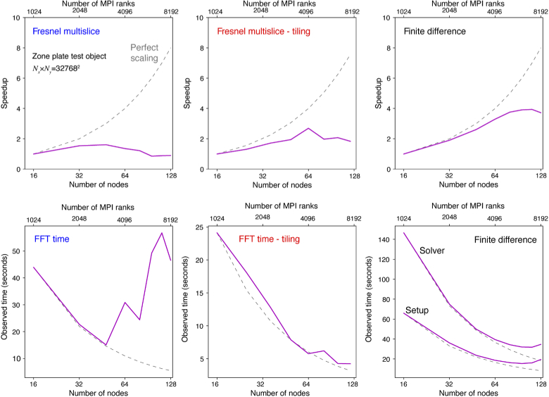
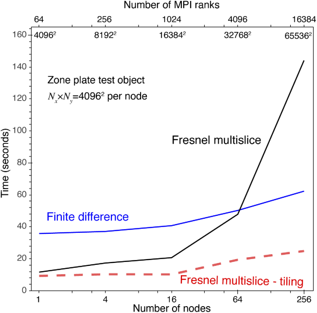
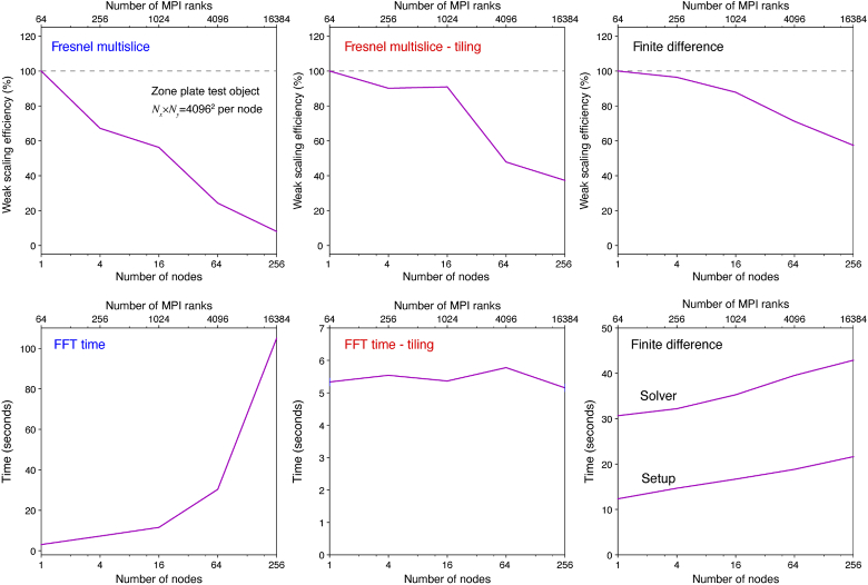
Calculations of X-ray wave propagation in large objects are needed for modeling diffractive X-ray optics and for optimization-based approaches to image reconstruction for objects that extend beyond the depth of focus. We describe three methods for calculating wave propagation with large arrays on parallel computing systems with distributed memory: (1) a full-array Fresnel multislice approach, (2) a tiling-based short-distance Fresnel multislice approach, and (3) a finite difference approach. We find that the first approach suffers from internode communication delays when the transverse array size becomes large, while the second and third approaches have similar scaling to large array size problems (with the second approach offering about three times the compute speed).

Fig. 1.

For tiling-based short-distance Fresnel multislice, one can use a tiling approach to split a large 2D array of dimension $N_x\times N_y$ into a set of smaller arrays, each of size $N_{x,\text{tile}}\times N_{y,\text{tile}}$, so that these smaller arrays can be processed on separate computational nodes. When doing so, one must add a buffer zone of physical width $r_2$ (Eq. (14)), and pixel width $N_{\text{buffer}}=r_2/{\mathrm{\Delta }}_x$ (Eq. (15)), to each side of the tile with information from neighboring tiles. This accounts for diffraction from features at the edge of nearby tiles coming into the field of view of the tile being processed.

Fig. 2.

Mean squared error of the exit wave of a subregion of a 3D object as a function of the buffer zone width $r_2=(w/\sqrt{2})\sqrt{\lambda z_{\text{prop}}}$ of Eq. (13), showing that the choice of $r_2=3.97\sqrt{\lambda z}$ of Eq. (14) gives good results (a mean squared error of ${10}^{-9}$ compared to a variance in the reference modulus of $4\times {10}^{-6}$). Shown here is the result of using tiling-based short-distance propagation through a ${256}^3$ voxel object as used in another publication [12]. The object was split into 4 $128\times 128$ tiles with the “seams” of the tiles running across the object, and buffer zones are added around each tile.

Fig. 3.

Illustration of the metric for measuring the RMS average $\overline{A}{\xi }_{\varphi }$ of the magnitude error at one pixel $i$ between the complex value before convergence ($A_{n,i}\exp [i{\varphi }_{n,i}]$; shown in blue) and after convergence ($A_{\mathrm{\infty },i}\exp [i{\varphi }_{\mathrm{\infty },i}]$; shown in red). When obtaining a particular measure of the phase difference ${\varphi }_{n,i}-{\varphi }_{\mathrm{\infty },i}$ from a complex value $\tilde{z}=A\exp [i\varphi ]$ on the real (Re) and imaginary (Im) plane, one could obtain erroneous values in the case shown where the phase before convergence is reported as $\pi -{ϵ}_{n,i}$ while the phase after convergence is reported as $-(\pi -{ϵ}_{\mathrm{\infty },i})$, one would obtain an erroneous phase difference ${\varphi }_{n,i}-{\varphi }_{\mathrm{\infty },i}$ of near $2\pi$. Calculating the RMS difference between complex wavefields (Eq. (24)) circumvents this problem by measuring the end-to-end distance between the red and blue vectors at individual pixels $i$, a result that does not require phase wrapping. When the moduli $A_{n,i}$ and $A_{\mathrm{\infty },i}$ are similar, the average modulus of the green vector (labeled here as $\overline{A}{\xi }_{\varphi }$ using Eq. (24)) is approximately linearly related to the RMS average of $\overline{A}|{\varphi }_{n,i}-{\varphi }_{\mathrm{\infty },i}|$ subtended by the blue and red vectors.

Fig. 4.

Fresnel zone plate test object, with a thickness $t$ and a finest zone width of $d{r}_N$. The beam propagation direction $\hat{z}$ is also indicated.

Fig. 5.

The process used to generate the porous aluminum phantom object (right). A larger scale tomographic reconstruction of an activated charcoal specimen (left) was used as the data source. From the 4198 tomographic reconstruction slices of $6613\times 6613$ pixels each, a $2448\times 2448\times 51$ voxel subregion was selected through all slices to avoid ring artifacts near the rotation axis. This subregion was then replicated into a $4\times 4$ grid in the plane of the object slices, with pyramid blending used at the tile overlaps and the edges blended out to vaccum (that is, to a specimen density of zero). The resulting $4096\times 4096\times 51$ voxel array was then rotated so that the original data rotation axis (veritcal, at left) became the beam propagation direction $\hat{z}$ in the phantom object at right, after which both the pixel size and the contrast of the object were modified to yield the porous aluminum phantom object.

Fig. 6.

Histogram of voxel densities of the porous aluminum test object. By setting the average occupancy of the charcoal test object to 1 and then multiplying by the refractive index of aluminum, the porous aluminum test object was inadvertently created with voxel densities exceeding the actual density of aluminum. This means that the test object was more strongly refracting than a true aluminum object would be, but this does not affect our measurement of the convergence or timing properties of the algorithms tested.

Fig. 7.

Convergence test for the three algorithms of Sec. 2 using the porous aluminum test object. For this test, the ${4096}^2$ transverse subarray of the object was selected, and the thickness $t=147.5$ $\mathrm{\mu }$m was bilinearly re-sampled onto a variable number of slices $N_z$. Using the convergence criterion of Eq. (26) giving a tolerance for this sample of ${[\overline{A}{\xi }_{\varphi }]}_{\text{Al}}=0.245$ (Eq. (30)), the full-array Fresnel multislice approach reached convergence with $n_C=84$ slices with ${\mathrm{\Delta }}_z=1.64$ $\mathrm{\mu }$m while the tiling-based short-distance Fresnel multislice approach required $n_C=90$ slices with ${\mathrm{\Delta }}_z=1.64$ $\mathrm{\mu }$m. The finite difference method required $n_C=352$ slices with ${\mathrm{\Delta }}_z=0.42$ $\mathrm{\mu }$m for this irregular object.

Fig. 8.

Convergence of the finite difference approach as a function of transverse array size for the porous aluminum object. As in Fig. 7, the indicated size of transverse array (ranging from ${512}^2$ to ${4096}^2$ pixels) was extracted from the object, and the total object thickness $t=147.5$ $\mathrm{\mu }$m was bilinearly sampled along the propagation direction $\hat{z}$ to vary $N_z$. For each array size, the minimum number of slices $n_C$ (Eq. (26)) was calculated using the convergence threshold ${[\overline{A}{\xi }_{\varphi }]}_{\text{Al}}=0.245$ of Eq. (30). As can be seen, the finite difference method converges more quickly with smaller transverse arrays, reaching $n_C=96$ (with slice thickness ${\mathrm{\Delta }}_z=1.54$ $\mathrm{\mu }$m) at ${512}^2$ transverse grid size with this irregular object.

Fig. 9.

Convergence test of the three algorithms for a Fresnel zone plate as a highly regular test object. In all cases, the zone plate thickness was $t=30.81$ $\mathrm{\mu }$m and the minimum zone width was $d{r}_N=20$ nm, but the diameter $d$ (and thus focal length $f$) of the zone plate was adjusted to match 80% of the transverse array size for ${4096}^2$, ${16384}^2$, and ${65536}^2$ transverse pixels, respectively. Using the convergence threshold ${[\overline{A}{\xi }_{\varphi }]}_{\text{zp}}=0.135$ (Eq. (28)) for this object to find the minimum number of slices $n_C$ (Eq. (26)), all three algorithms had minimum slice numbers $n_C$ that were independent of transverse array size and that were within a factor of 2 of the thickness $z_{\text{K-C}}=2.3$ $\mathrm{\mu }$m (Eq. (11)) at which waveguide effects would be expected for this specimen. The finite difference method required fewer slices with $n_C=8$ and ${\mathrm{\Delta }}_z=3.85$ $\mathrm{\mu }$m, while the two Fresnel multislice methods required slightly more slices ($n_C=21$ and ${\mathrm{\Delta }}_z=1.47$ $\mathrm{\mu }$m for full-array Fresnel multislice, and $n_C=23$ and ${\mathrm{\Delta }}_z=1.34$ $\mathrm{\mu }$m for tiling-based short-distance Fresnel multislice).

Fig. 10.

Time for calculating the exit wave from the zone plate test object as a function of the number of nodes used. This “strong scaling” test was done with a constant transverse grid size of $N_x\times N_y={32768}^2$ pixels on the computational cluster “theta” (see Table 1), and using the number of slices $n_C$ each algorithm required for convergence to the error tolerance ${[\overline{A}{\xi }_{\varphi }]}_{\text{zp}}$ of Eq. (28) (the resulting values of $n_C$ were consistently within 1 or 2 slices of the values shown in Fig. 9). While the finite difference method takes the longest amount of time with a small number of nodes, it benefits the most from increased parallelization so that the calculation time drops significantly by the time 128 nodes are employed. The full-array Fresnel multislice method shows only a modest time decrease as more nodes are employed, until at 64 nodes the calculation time begins to increase due to the requirement for considerable data communication between nodes. Because the tiling-based short-distance Fresnel multislice approach allows each node to proceed through to the exit wave plane before inter-node communication is again required, it takes the least time but after 64 nodes one again sees a slight increase in calculation time if additional nodes are used. Note that 64 nodes corresponds to a transverse array size of 4096² pixels per node. Further details on this “strong scaling” test are provided in Fig. 11.

Fig. 11.

Further details on the “strong scaling” test results shown in Fig. 10. These tests were of the zone plate test object on a $N_x\times N_y={32768}^2$ pixel transverse grid. For each of the three calculation methods, we show at top the speedup versus the number of nodes used (with a a linear “perfect scaling” trend showing up as a curved line on this log-linear plot). This shows that the finite difference method has the best scaling to calculation speedup with increased number of nodes. At bottom we show the time required for key operations in the various methods: the time required for a fast Fourier transform (FFT) in the full-array Fresnel multislice and tiling-based short-distance Fresnel multislice methods, and the time for problem setup and then problem solution for the finite difference method. With the full-array FFT approach, the advantage of having more processors is outweighed by data communication overhead when 64 or more nodes are used.

Fig. 12.

Time for calculating the exit wave for the zone plate test object as a function of increasing the transverse array size along with the number of nodes, with each node given a transverse grid size of $N_x\times N_y={4096}^2$ (leading to a net array size of ${65536}^2$ for 256 nodes, as indicated just below the top of the plot). For each algorithm, the number of slices $n_C$ was as required for convergence to the error tolerance ${[\overline{A}{\xi }_{\varphi }]}_{\text{zp}}$ of Eq. (28), giving values of $n_C$ that were in all cases within 1 or 2 slices of the values shown in Fig. 9. This “weak scaling” test shows that both the finite difference and tiling-based short-distance Fresnel multislice approaches scale well as the problem size increases with the number of nodes used, consistent with the “strong scaling” test results of Fig. 10. With the full-array Fresnel multislice approach, the time required for data communication between nodes for full-array FFTs means that even with many nodes available large problems require considerably more time to compute.

Fig. 13.

Further details on the “weak scaling” test results shown in Fig. 12. These tests were of the zone plate test object with a constant array size of $N_x\times N_y={4096}^2$ per node, leading to a net array size of ${65536}^2$ for 256 nodes. The top row shows the scaling efficiency for each of the three algorithms, which is the completion time compared to the 1 node result divided by the number of nodes used. The bottom row shows the time for key operations in each method: a fast Fourier transform or FFT for the Fresnel multislice approaches, and problem setup and solution for the finite difference method. As can be seen, the full-array Fresnel multislice approach has especially poor “weak scaling” performance due to the need for internode communcation at each slice position, while the tiling-based short-distance Fresnel multislice approach offers better parallel performance. The finite difference approach takes a longer time, but with less of a decrease in efficiency for larger transverse array size.

References

1. Eriksson M., van der Veen J. F., Quitmann C., “Diffraction-limited storage rings – a window to the science of tomorrow,” J. Synchrotron Radiat. 21(5), 837–842 (2014).10.1107/S1600577514019286 - DOI - PubMed
1. Born M., Wolf E., Principles of Optics (Cambridge University Press, Cambridge, 1999), seventh ed.
1. Jacobsen C., X-ray Microscopy (Cambridge University Press, Cambridge, 2020).
1. Van den Broek W., Koch C. T., “Method for retrieval of the three-dimensional object potential by inversion of dynamical electron scattering,” Phys. Rev. Lett. 109(24), 245502 (2012).10.1103/PhysRevLett.109.245502 - DOI - PubMed
1. Ren D., Ophus C., Chen M., Waller L., “A multiple scattering algorithm for three dimensional phase contrast atomic electron tomography,” Ultramicroscopy 208, 112860 (2020).10.1016/j.ultramic.2019.112860 - DOI - PubMed