Ecological limits to evolutionary rescue

Abstract

Environments change, for both natural and anthropogenic reasons, which can threaten species persistence. Evolutionary adaptation is a potentially powerful mechanism to allow species to persist in these changing environments. To determine the conditions under which adaptation will prevent extinction (evolutionary rescue), classic quantitative genetics models have assumed a constantly changing environment. They predict that species traits will track a moving environmental optimum with a lag that approaches a constant. If fitness is negative at this lag, the species will go extinct. There have been many elaborations of these models incorporating increased genetic realism. Here, we review and explore the consequences of four ecological complications: non-quadratic fitness functions, interacting density- and trait-dependence, species interactions and fundamental limits to adaptation. We show that non-quadratic fitness functions can result in evolutionary tipping points and existential crises, as can the interaction between density- and trait-dependent mortality. We then review the literature on how interspecific interactions affect adaptation and persistence. Finally, we suggest an alternative theoretical framework that considers bounded environmental change and fundamental limits to adaptation. A research programme that combines theory and experiments and integrates across organizational scales will be needed to predict whether adaptation will prevent species extinction in changing environments. This article is part of the theme issue 'Integrative research perspectives on marine conservation'.

Keywords: climate change; eco-evolutionary dynamics; environmental change; evolutionary rescue; moving optimum; quantitative genetics.

Figure 1.

Overview of classical quantitative genetics moving optimum models, with fitness landscape r(x). (a) The species adapts at a rate proportional to the fitness gradient $\mathrm{\partial }\overline{r}/\mathrm{\partial }\overline{x}$, while the optimal trait E increases at rate δ, shifting the entire fitness landscape. (b) An equivalent formulation in the moving frame of reference considers the dynamics of the trait lag x_l = E−x, where the moving optimum acts directly on the trait lag. The trait lag reaches an equilibrium ${\hat{x}}_{\mathrm{l}}$. (c) The equilibrium trait lag increases with increasing δ. (d) When the equilibrium trait lag exceeds the critical value x_l,c where fitness is zero, the species cannot keep up with environmental change and is driven extinct. (Online version in colour.)

Figure 2.

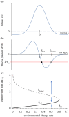
Non-quadratic fitness landscapes. (a) A Gaussian fitness landscape. (b) The fitness gradient has extrema at the inflection points of the fitness landscape, so that the rate of adaptation does not increase linearly with trait lag. (c) Depending on the rate of environmental change δ and the additive genetic variance V_g, this results in either two equilibria, one stable ${\hat{x}}_{\mathrm{l},\mathrm{st}}$ (solid line) and one unstable ${\hat{x}}_{\mathrm{l},\mathrm{unst}}$ (dashed line), or no equilibrium at all when δ > δ_tip. Parameter values: r_max = 1, σ_r = 1, d = 0.1, V_g = 1. (Online version in colour.)

Figure 3.

Interaction between density dependence (DD) and trait dependence (TD) of fitness. (a) When density and trait dependence enter different terms, they do not interact and the equilibrium trait lag increases linearly with δ. (b) When births are both density- and trait-dependent, the equilibrium trait lag increases nonlinearly with δ but results in the same critical value δ_c. (c) When deaths are both density- and trait-dependent, the species may continue to persist for δ_c < δ < δ_tip with two stable equilibria (solid lines), separated by an unstable equilibrium (dashed line). Parameter values: d_min = 0.1 or d = 0.1, b_max = 1 or b = 1, σ_r = 1, V_g = 1. (Online version in colour.)

Figure 4.

Eco-evo phase plane analysis of density- and trait-dependent death model. (a) For δ < δ_c, there is a single stable equilibrium (filled circle) where the species persists. (b) For δ_c < δ < δ_tip, there are two stable equilibria (persistence and extinction) separated by an unstable equilibrium (open circle). (c) For δ > δ_tip, only the extinction equilibrium is stable. Other parameter values as in figure 3.

Figure 5.

Contrasting (a) the moving optimum paradigm with (b) finite fitness landscapes with bounded environmental change. In (a), indefinite species persistence occurs when the equilibrium trait lag is less than the critical lag. In (b), the species can persist without evolution when the final environmental condition E_post < E_c,eco, goes extinct even with evolution when E_post > E_c,evo and may or may not persist when E_c,eco < E_post < E_c,evo.

Figure 6.

When E_c,eco < E_post < E_c,evo, persistence depends on the amount of additive genetic variance V_g relative to the rate of environmental change. (a) When change is slow relative to the rate of adaptation, fitness remains positive and the population maintains a high abundance. (b) For smaller genetic variance, the transient trait lag increases, putting populations at risk. (c) When the trait lag leaves the region of positive growth, the population can reach low densities where demographic stochasticity may drive it extinct. Fitness function r(x,E) = 1−(x−E)²−0.75E, environmental dynamics E(t) = 6(δt)⁵−15(δt)⁴ + 10(δt)³ for δt < 1 and E(t) = E_post = 1 for δt < 1. Mortality is density-dependent. Parameter values: δ = 0.1, d = 0.1.

References

1. Bell G. 2017. Evolutionary rescue. Annu. Rev. Ecol. Evol. Syst. 48, 605–627. (10.1146/annurev-ecolsys-110316-023011) - DOI
1. Radchuk V, et al. 2019. Adaptive responses of animals to climate change are most likely insufficient. Nat. Commun. 10, 3109 (10.1038/s41467-019-10924-4) - DOI - PMC - PubMed
1. Kopp M, Matuszewski S. 2014. Rapid evolution of quantitative traits: theoretical perspectives. Evol. Appl. 7, 169–191. (10.1111/eva.12127) - DOI - PMC - PubMed
1. Aitken SN, Yeaman S, Holliday JA, Wang T, Curtis-McLane S. 2008. Adaptation, migration or extirpation: climate change outcomes for tree populations. Evol. Appl. 1, 95–111. (10.1111/j.1752-4571.2007.00013.x) - DOI - PMC - PubMed
1. Willi Y, Hoffmann AA. 2009. Demographic factors and genetic variation influence population persistence under environmental change. J. Evol. Biol. 22, 124–133. (10.1111/j.1420-9101.2008.01631.x) - DOI - PubMed
Publication types
LinkOut - more resources