. 2018 May:104:138-166.
doi: 10.1016/j.euroecorev.2018.02.005. Epub 2018 Mar 11.

Marriage and Health: Selection, Protection, and Assortative Mating

Affiliations

Marriage and Health: Selection, Protection, and Assortative Mating

Nezih Guner et al. Eur Econ Rev. 2018 May.

Abstract

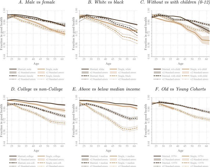
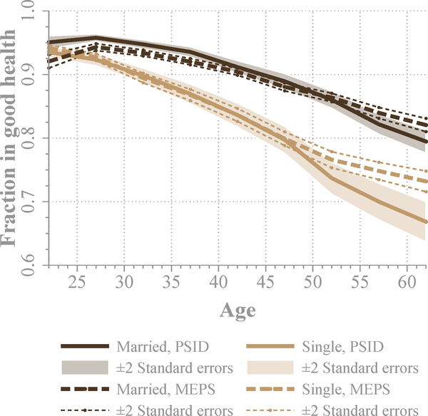
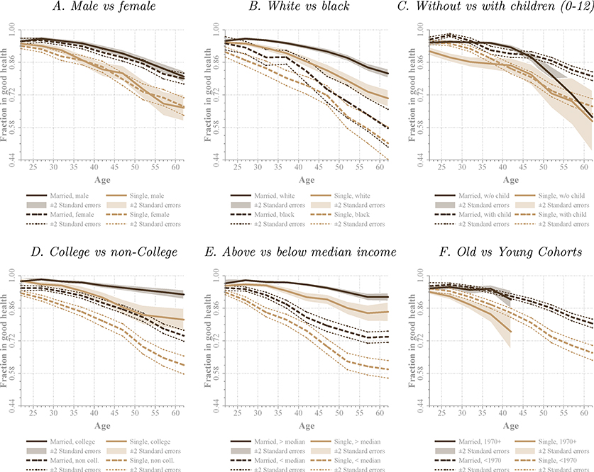
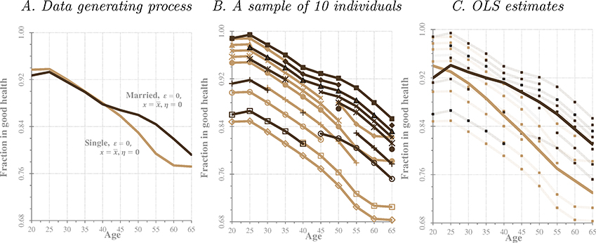
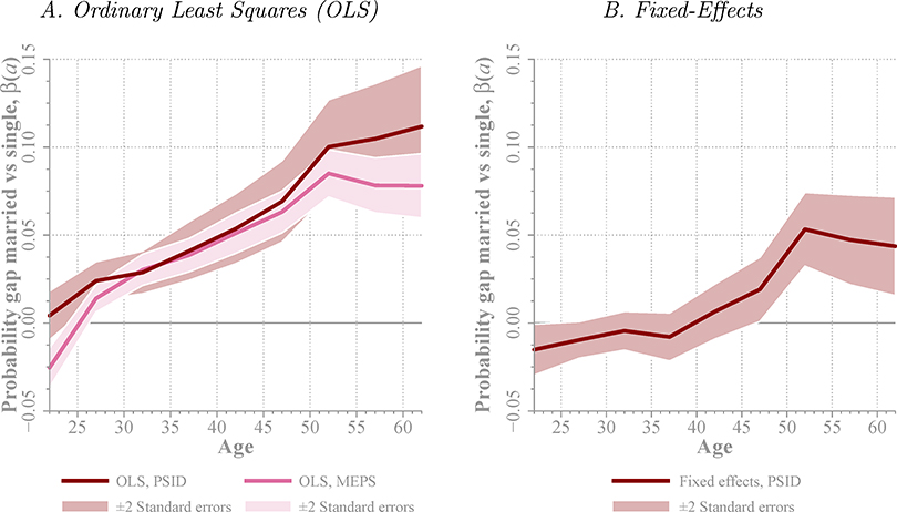
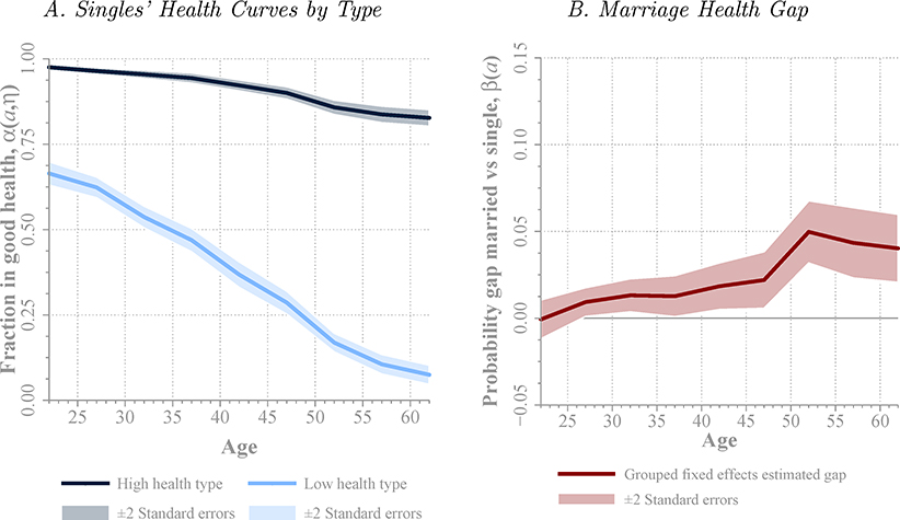
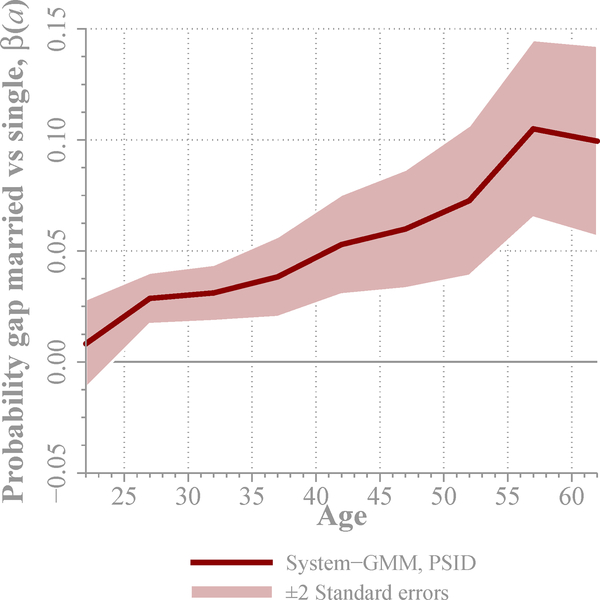
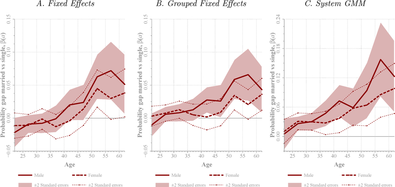
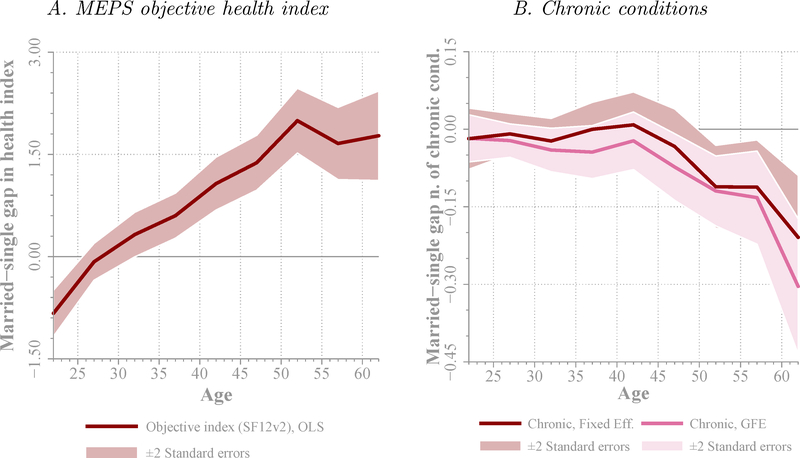
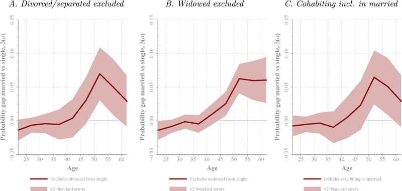
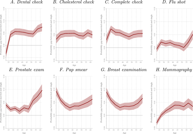
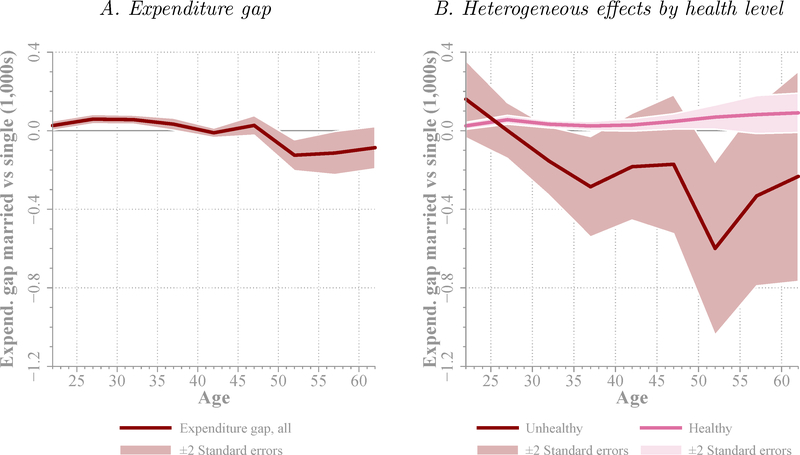
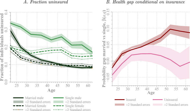
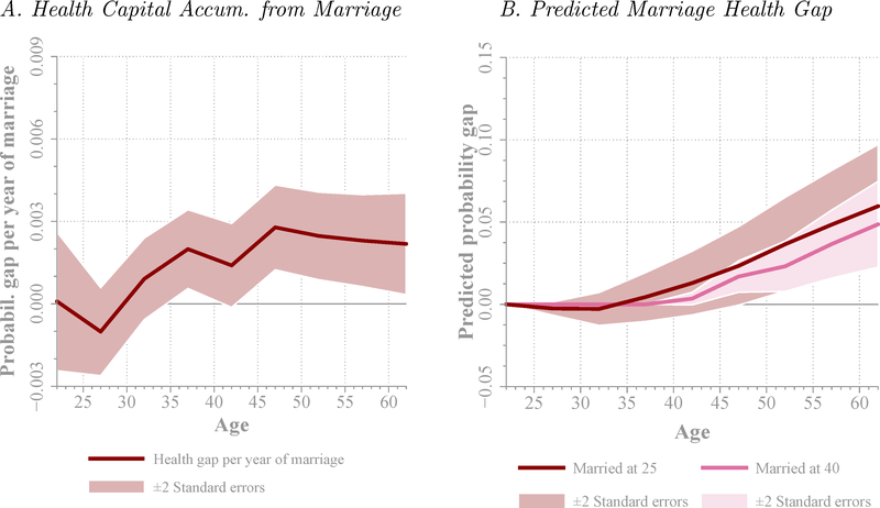
Using data from the Panel Study of Income Dynamics (PSID) and the Medical Expenditure Panel Survey (MEPS), we analyze the health gap between married and unmarried individuals of working-age. Controlling for observables, we find a gap that peaks at 10 percentage points at ages 55-59 years. The marriage health gap is similar for men and women. If we allow for unobserved heterogeneity in innate health (permanent and age-dependent), potentially correlated with timing and likelihood of marriage, we find that the effect of marriage on health disappears below age 40 years, while about 5 percentage points difference between married and unmarried individuals remains at older ages (55-59 years). This indicates that the observed gap is mainly driven by selection into marriage at younger ages, but there might be a protective effect of marriage at older ages. Exploring the mechanisms behind this result, we find that better innate health is associated with a higher probability of marriage and a lower probability of divorce, and there is strong assortative mating among couples by innate health. We also find that married individuals are more likely to have a healthier behavior compared to unmarried ones. Finally, we find that health insurance is critical for the beneficial effect of marriage.

Keywords: Assortative Mating; Grouped-Fixed-Effects Estimator; Health; I10; I12; Innate Health; J10; Marriage; Panel Data; Protective Effect of Marriage.


Figures

Figure B1.
Figure B1.. Health and Marital Status, Different Socioeconomic Groups (MEPS)
Note: This figure reproduces the results in Figure 2 using the MEPS sample. Plotted lines represent the weighted fraction of married and unmarried individuals that report being healthy. Fractions are reported, as indicated, for male and female, white and black, without and with children aged 0–12 living in the household, college graduates and non-college, above and below median income, and born after and before 1970. The horizontal axis indicates age, which is grouped in five-year categories (20–24 through 60–64). Confidence bands of ± two standard errors are computed using sample stratification design.
Figure 1.
Figure 1.. Health and Marital Status (PSID and MEPS)
Note: Plotted lines represent the weighted fraction of married and unmarried individuals that report being healthy, computed using the PSID and the MEPS. The horizontal axis indicates age, which is grouped in five-year categories (20–24 through 60–64). Confidence bands of ± two standard errors are computed according to the corresponding survey design: sample weights are used for the PSID, and Taylor linearized standard errors are computed for the MEPS. PSID standard errors are clustered at the household level.
Figure 2.
Figure 2.. Health and Marital Status for Different Socioeconomic Groups
Note: Plotted lines represent the weighted fraction of married and unmarried individuals that report being healthy, obtained from the PSID. Fractions are reported, as indicated, for male and female, white and black, without and with children aged 0–12 living in the household, college graduates and non-college, above and below median income, and born after and before 1970. The horizontal axis indicates age, which is grouped in five-year categories (20–24 through 60–64). Confidence bands of ± two standard errors are computed using sample weights. Standard errors are clustered a the household level.
Figure 3.
Figure 3.. Unobserved Heterogeneity and the Self-Selection Bias: An Example
Note: This figure illustrates the bias from omitting unobserved heterogeneity in the estimation of the health curves. Panel A presents the data generating process. Married health curves are dark and single health curves are light. Panel B plots a hypothetical sample of 10 individuals simulated from the data generating process, all of them with x=x¯ and ε = 0. Types of markers identify individuals. Panel C shows OLS estimates of the married and single curves on the simulated sample.
Figure 4.
Figure 4.. Marriage Health Gap: OLS and Fixed-Effects Estimation Results
Note: Solid lines show estimated marriage health gaps β(a) from Equation (1). The regression is fitted to the PSID and the MEPS. Left figure presents estimates from OLS regressions, and right figure presents fixed-effects estimates. The dependent variable is an indicator variable that takes a value of one if the individual is healthy. Control variables include female, black, and college dummies, income, dummies for 0–3, 4–12, and 13–18 year-old children at home, and year of birth dummies; regressions also estimate α(a). The horizontal axis indicates age. In estimation, five-year age bins (20–24, through 60–64) are considered. The center point of the bin is represented in the figure. Weights are used in estimation. Confidence bands of ± two standard errors around point estimates are computed following the survey design of each database. Standard errors are clustered at the household level in the PSID.
Figure 5.
Figure 5.. Marriage Health Gap: Grouped-Fixed-Effects Estimation Results
Note: Left plot shows α(a, ηg), the estimated health curves for unmarried individuals of high and low health types, and the right plot shows β(a), the estimated marriage health gap, both of them from Equation (2). The model is fitted to the PSID, implementing the algorithm described in Bonhomme and Manresa (2015) for two types. The algorithm was started from 1,000 different random points, and it generally converged to the same minimum. It identified 81.3% healthy-type individuals (12,660), and 18.7% of unhealthy-type (2,909). The dependent variable is an indicator variable that takes the value of one if the individual is healthy. Control variables include female, black, and college dummies, income, dummies for 0–3, 4–12, and 13–18 year-old children at home, and year of birth dummies. The horizontal axis indicates age. In estimation, five-year age bins (20–24, through 60–64) are considered. The center point of the bin is represented in the figure. Weights are used in estimation. Confidence bands of ± two standard errors are computed clustering standard errors at the household level.
Figure 6.
Figure 6.. Marriage Health Gap: System-GMM Estimation Results
Note: The solid line shows the estimated marriage health gap β(a) from the dynamic model in Equation (3). The regression is estimated by System-GMM (Arellano and Bover, 1995) from the PSID for the subperiod 1985–1997. The dependent variable is an indicator variable that takes a value of one if the individual is healthy. Control variables include the lagged dependent variable and a vector of controls that includes female, black, and college dummies, income, dummies for 0–3, 4–12, and 13–18 year-old children at home, and year of birth dummies; regressions also estimate α(a). The horizontal axis indicates age. In estimation, five-year age bins (20–24, through 60–64) are considered. The center point of the bin is represented in the figure. Weights are used in estimation. Confidence bands of ± two standard errors are computed clustering at the household level.
Figure 7.
Figure 7.. Marriage Health Gap: Results by Gender
Note: Solid lines show estimated marriage health gaps β(a) from Equations (1), (2), and (3) respectively, estimated separately on the samples of males and females. The regression is fitted to the PSID. The dependent variable is an indicator variable that takes a value of one if the individual is healthy. Control variables include black and college dummies, income, dummies for 0–3, 4–12, and 13–18 year-old children at home, and year of birth dummies. The regressions also estimate α(a), α(a, ηgi), and φhit−1 + α(a) respectively. The horizontal axis indicates age. In estimation, five-year age bins (20–24, through 60–64) are considered. The center point of the bin is represented in the figure. Weights are used in estimation. Confidence bands of ± two standard errors around point estimates are computed following the survey design of each database. Standard errors are clustered at the household level in the PSID.
Figure 8.
Figure 8.. Alternative Health Measures
Note: Plotted lines show the estimated marriage health gaps β(a) for two alternative measures of health: SF12v2 objective index of health (left), estimated by OLS from the MEPS, and the cumulative number of different chronic conditions suffered by the individual (right), which includes fixed-effects estimates and group fixed effects estimates as indicated, both obtained from the PSID for the subperiod 1999–2013. The following chronic conditions are considered: stroke, heart attack, hypertension, diabetes, cancer, lung disease, arthritis, asthma, memory loss, and learning disorder, as defined in the PSID. Group fixed effects estimates from the right plot are obtained implementing the algorithm described in Bonhomme and Manresa (2015) for two types. The algorithm was started from 1,000 different random points, and in general converged to the same global minimum. The algorithm identified 63% hightype individuals (9,804), and 37% of low-type (5,765). Control variables include female, black, and college dummies, income, dummies for 0–3, 4–12, and 13–18 year-old children at home, and year of birth dummies; regressions also estimate α(a) or α(a, ηg). The horizontal axis indicates age. In estimation, five-year age bins (20–24, through 60–64) are considered. The center point of the bin is represented in the figure. Confidence bands of ± two standard errors around point estimates are computed following the survey design of each database. Standard errors are clustered at the household level in the PSID.
Figure 9.
Figure 9.. Alternative Definitions of Married and Single
Note: Solid lines show within-groups estimated marriage health gaps β(a) from Equation (1) for different definitions of married and unmarried populations: excluding divorced/separated or widowed from the sample, and including cohabitants in the married group, as indicated. The regression is fitted to the PSID. Control variables include female, black, and college dummies, income, dummies for 0–3, 4–12, and 13–18 year-old children at home, and year of birth dummies; regressions also estimate α(a). The horizontal axis indicates age. In estimation, five-year age bins (20–24, through 60–64) are considered. The center point of the bin is represented in the figure. Weights are used in estimation. Confidence intervals of ± two standard errors are computed clustering at the household level.
Figure 10.
Figure 10.. Preventive Health Checks and Marital Status
Note: Plotted lines show OLS estimates of the marriage gap in the probability of doing preventive checks. These differential curves are obtained from a regression that is similar to (1) but where the dependent variable is an indicator variable that takes the value of one if the individual did the indicated preventive check in previous years. The following preventive checks are considered: dental check at least once every year; cholesterol check, general physical examination, flu shot, prostate examination, Pap smear, breast examination, and mammography at least once in the last two years. The equation is fitted to data from the MEPS. Control variables include female, black, and college dummies, income, dummies for 0–3, 4–12, and 13–18 year-old children at home, and year of birth dummies, as well as current health, health insurance (public and private insurance dummies) and total health expenditures; regressions also estimate probability curve for singles. Weights are used in the estimation. The horizontal axis indicates age. In estimation, five-year age bins (20–24 through 60–64) are considered. The center point of the bin is represented in the figure. Dotted lines indicate ± two standard errors confidence bands around point estimates, which are Taylor linearized using survey stratification design in the MEPS.
Figure 11.
Figure 11.. Median Health Expenditures and Marital Status
Note: Solid line in the left plot shows the marriage gap in median health expenditures obtained from a regression to Equation (1), but with total health expenditures as the dependent variable. Solid lines in the right plot shows estimated heterogeneous marriage gaps in median expenditures by health level (healthy, dark blue, and unhealthy, light blue). Control variables include female, black, and college dummies, income, dummies for 0–3, 4–12, and 13–18 year-old children at home, and year of birth dummies, as well as health insurance (public and private insurance dummies); regressions also estimate median expenditure curves for singles in each health level. The regressions are estimated from the MEPS. The horizontal axis indicates age. In estimation, five-year age bins (20–24 through 60–64) are considered. The center point of the bin is represented in the figure. Dotted lines represent ± two bootstrapped standard error confidence bands.
Figure 12.
Figure 12.. Health Insurance, Health, and Marital Status
Note: Thick lines in the left plot show the weighted fraction of married and unmarried males and females that are not covered by any health insurance (public or private). Solid lines in the right plot are OLS estimates of the marriage health gap for insured and uninsured individuals. Results are obtained from the MEPS. In the right figure, control variables include female, black, and college dummies, income, dummies for 0–3, 4–12, and 13–18 year-old children at home, and year of birth dummies; regressions also estimate health curves for singles with and without insurance. The horizontal axis indicates age. In estimation, age is grouped in five-year bins (20–24 through 60–64) and the center point of the bin is graphed. Dotted lines indicate ± two standard errors confidence bands around point estimates, which are Taylor linearized computed following the survey stratification design.
Figure 13.
Figure 13.. Health Accumulation Through Marriage
Note: The left figure shows fixed-effect estimates of the health capital accumulated from marriage from a modified version of equation (1) in which the married dummy m is replaced by the number of years an individual have been married (zero if never married). Estimates are done with the PSID. The right figure plots the predicted marriage health gap for individuals married at age 25 and at age 40. Control variables include female, black, and college dummies, income, dummies for 0–3, 4–12, and 13–18 year-old children at home, and year of birth dummies; regressions also estimate the health curve for singles. The horizontal axis indicates age. In estimation, five-year age bins (20–24 through 60–64) are considered and the center point of the bin is graphed. Dotted lines are ± two standard errors confidence bands around point estimates, clustered at the household level.

Similar articles

Cited by

References

    1. Adams Peter, Hurd Michael D., McFadden Daniel, Merrill Angela, and Ribeiro Tiago, “Healthy, wealthy, and wise? Tests for direct causal paths between health and socioeconomic status,” Journal of Econometrics, January 2003, 112 (1), 356.
    1. Agency of Healthcare Research and Quality, “Medical Expenditure Panel Survey,” household component, public use data set. Produced and Distributed by The Agency for Healthcare Research and Quality 2011.
    1. Aizer Ayal A., Chen Ming-Hui, McCarthy Ellen P., Mendu Mallika L., Koo Sophia, Wilhite Tyler J., Graham Powell L., Choueiri Toni K., Hoffman Karen E., Martin Neil E., Hu Jim C., and Nguyen Paul L., “Marital Status and Survival in Patients With Cancer,” Journal of Clinical Oncology, November 2013, 31 (31), 3869–3876. - PMC - PubMed
    1. Anderson Michael, Dobkin Carlos, and Gross Tal, “The Effect of Health Insurance Coverage on the Use of Medical Services,” American Economic Journal: Economic Policy, February 2012, 4 (1), 1–27.
    1. Arellano Manuel and Bover Olympia, “Another Look at the Instrumental Variable Estimation of Error-Components Models,” Journal of Econometrics, July 1995, 68 (1), 29–51.

LinkOut - more resources