Simultaneous cortex-wide fluorescence Ca2+ imaging and whole-brain fMRI

Abstract

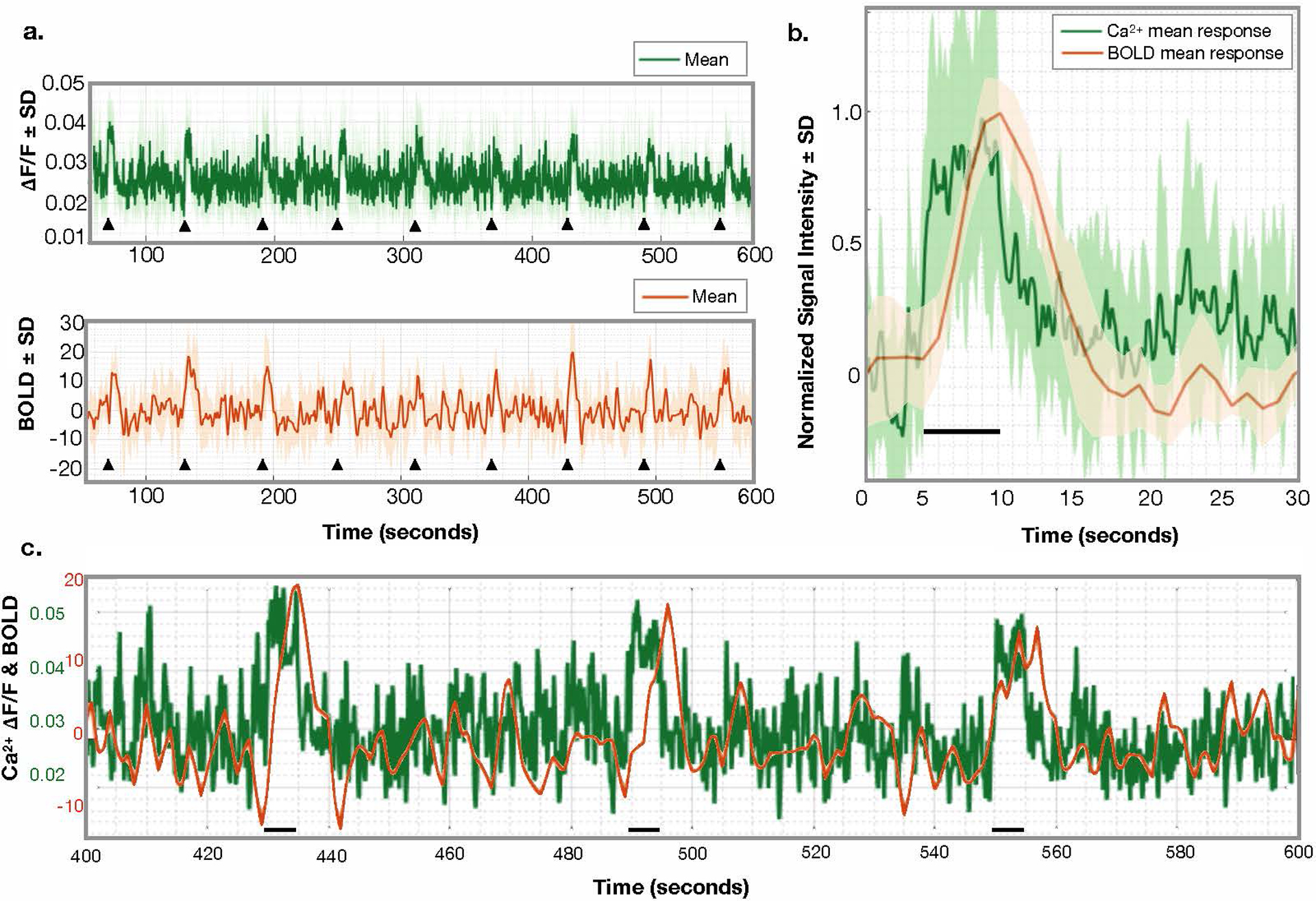
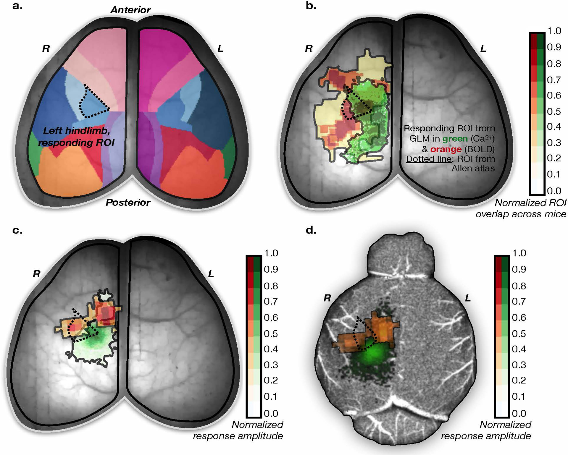
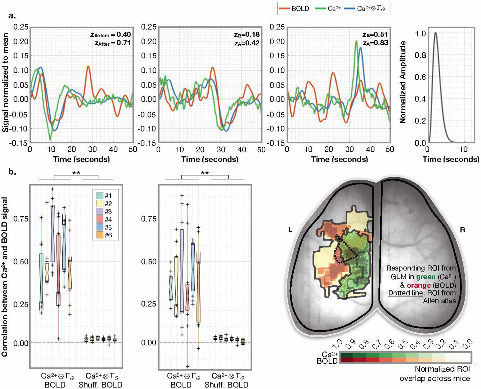
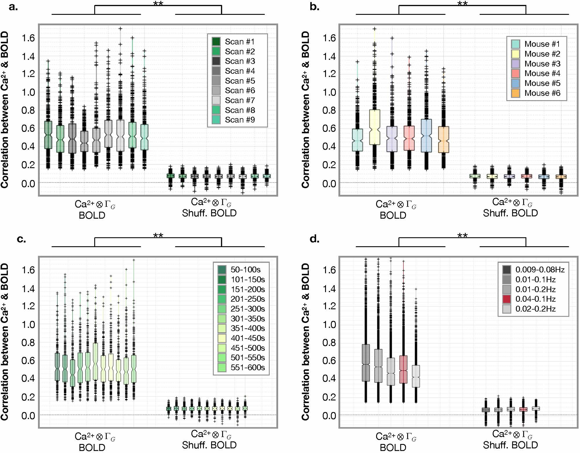
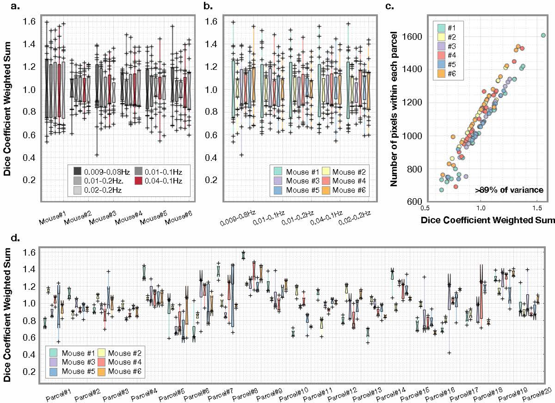
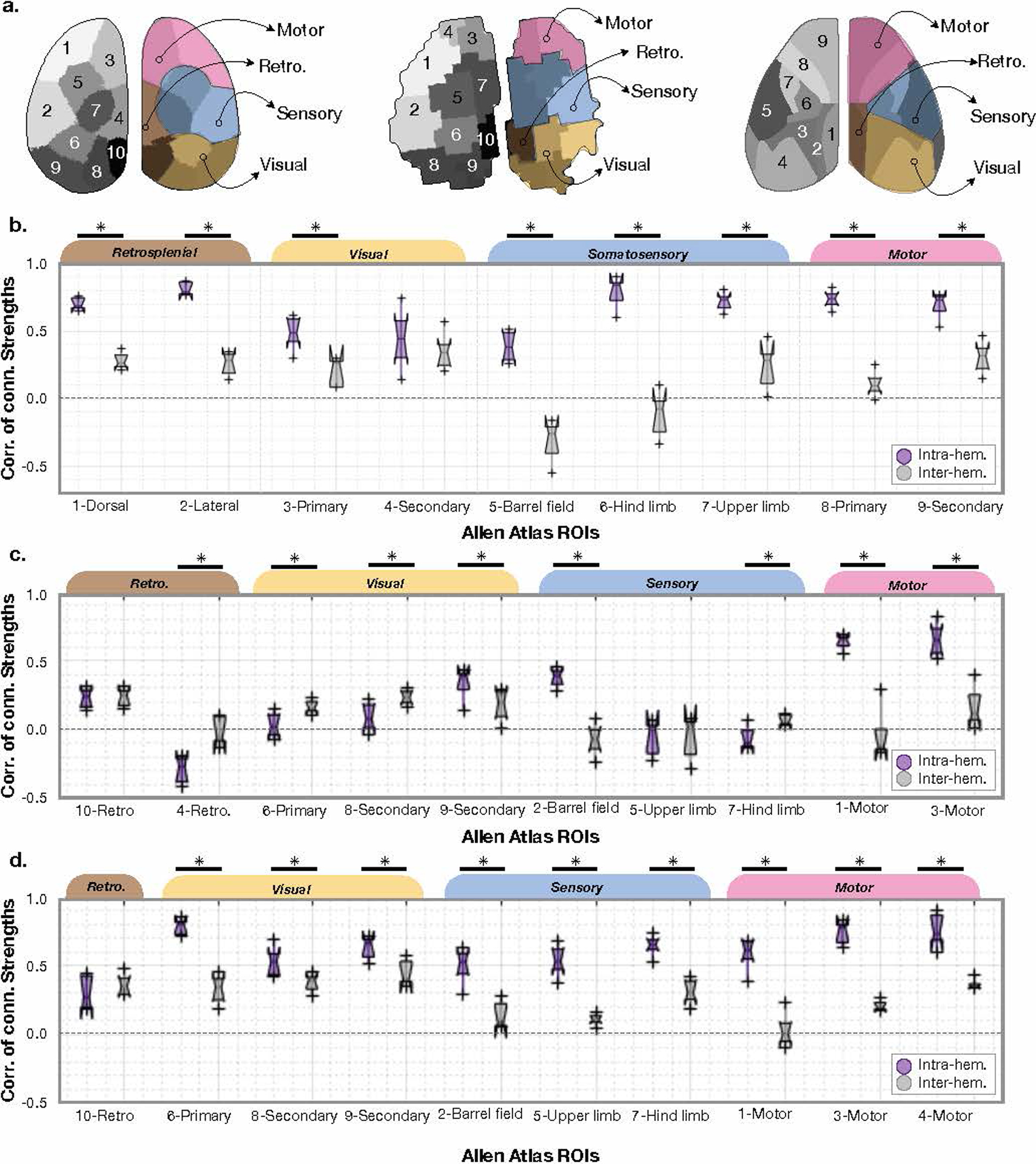
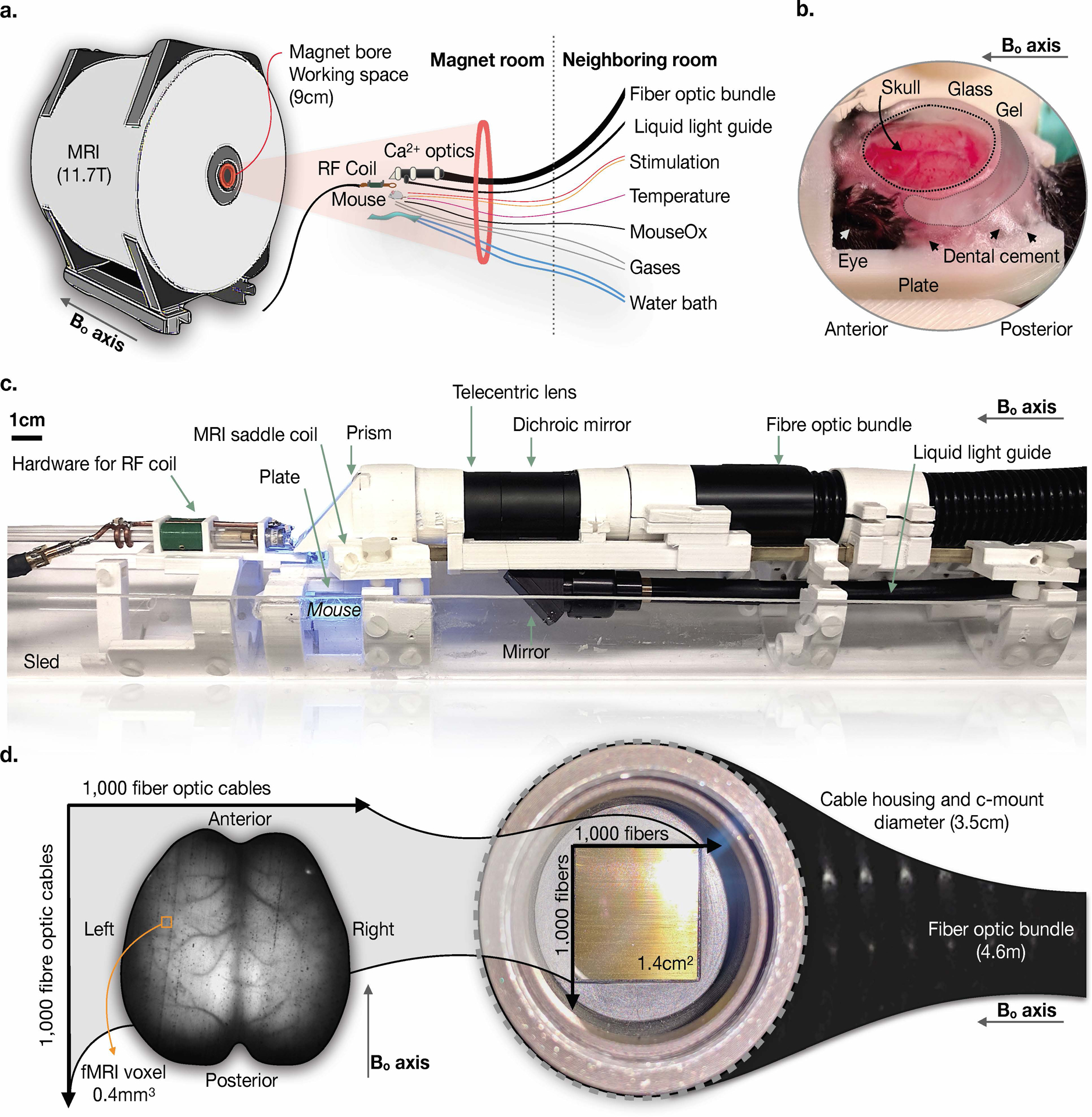
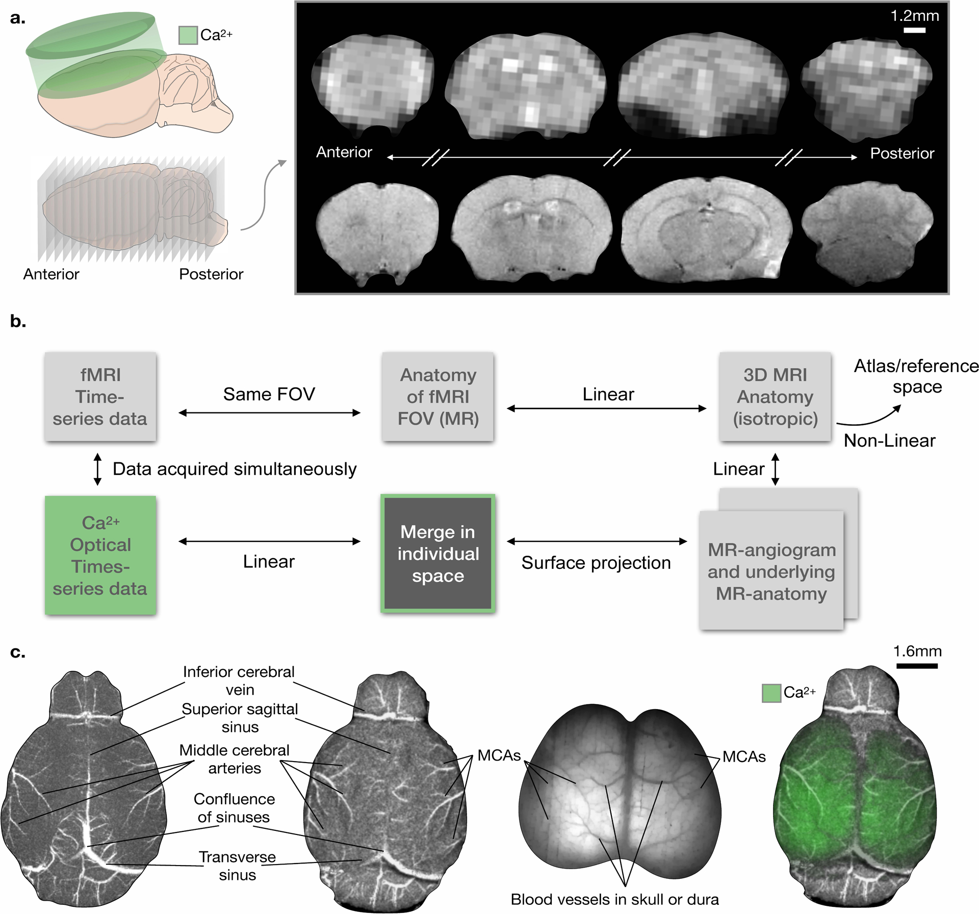
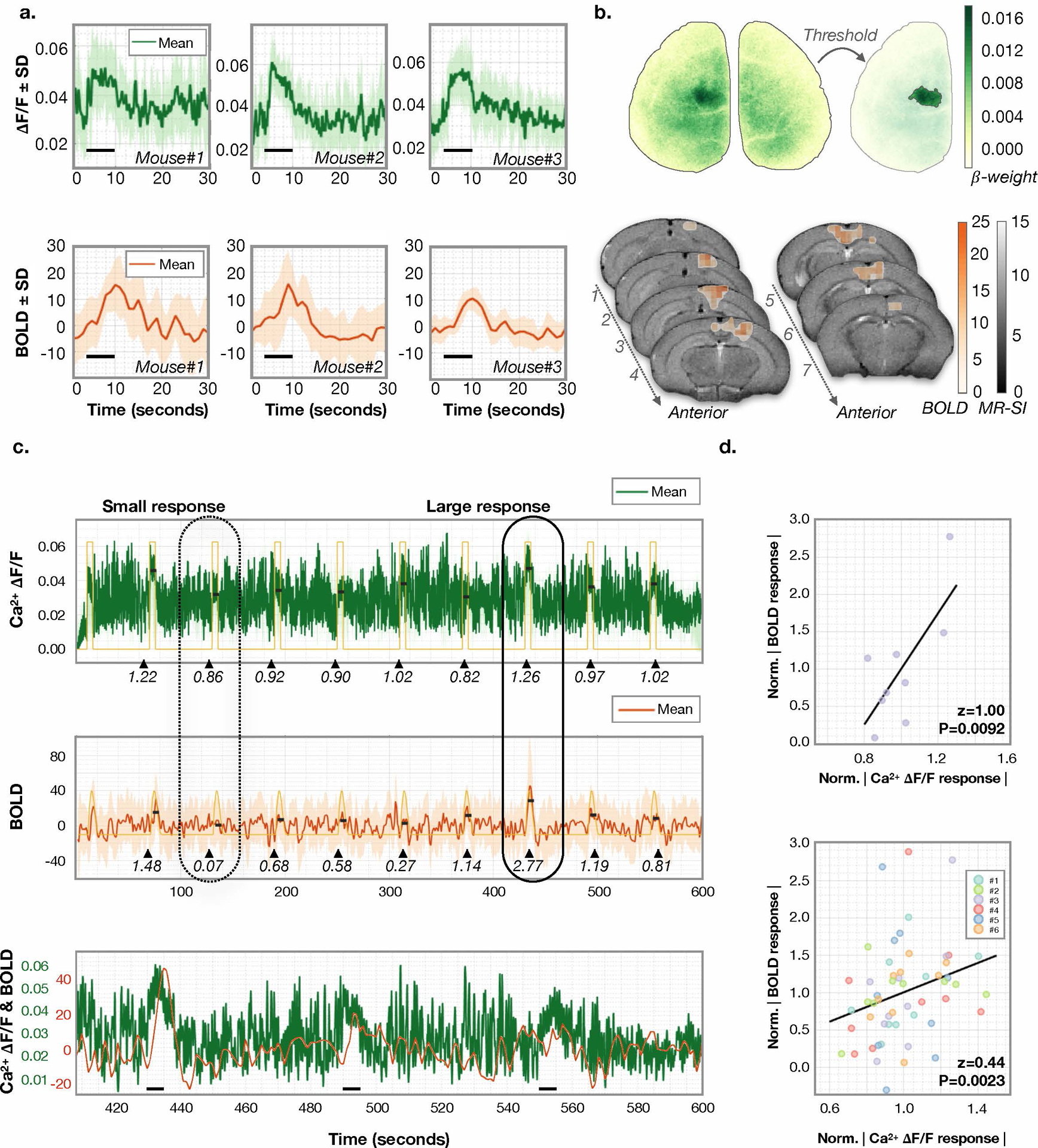
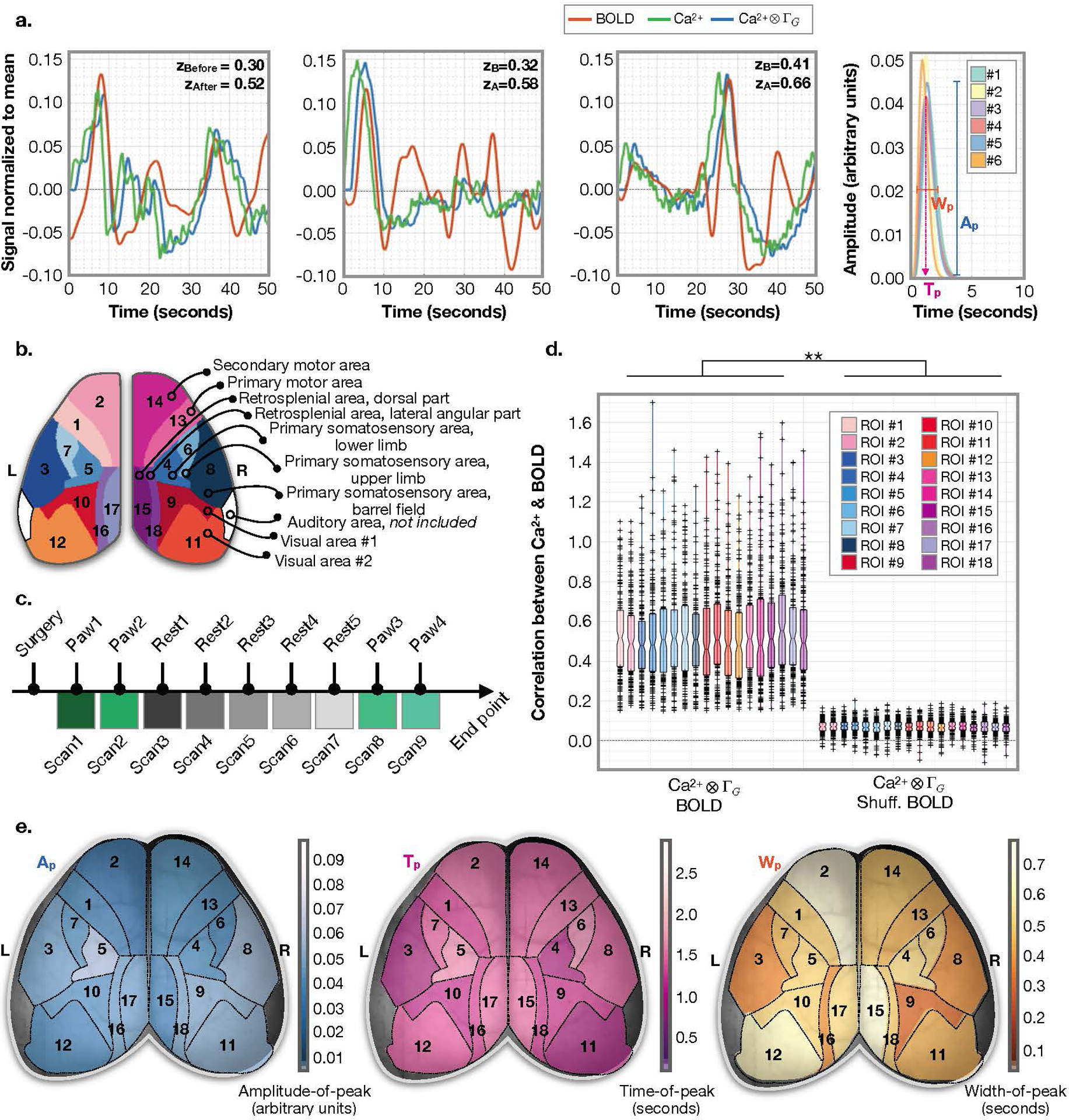
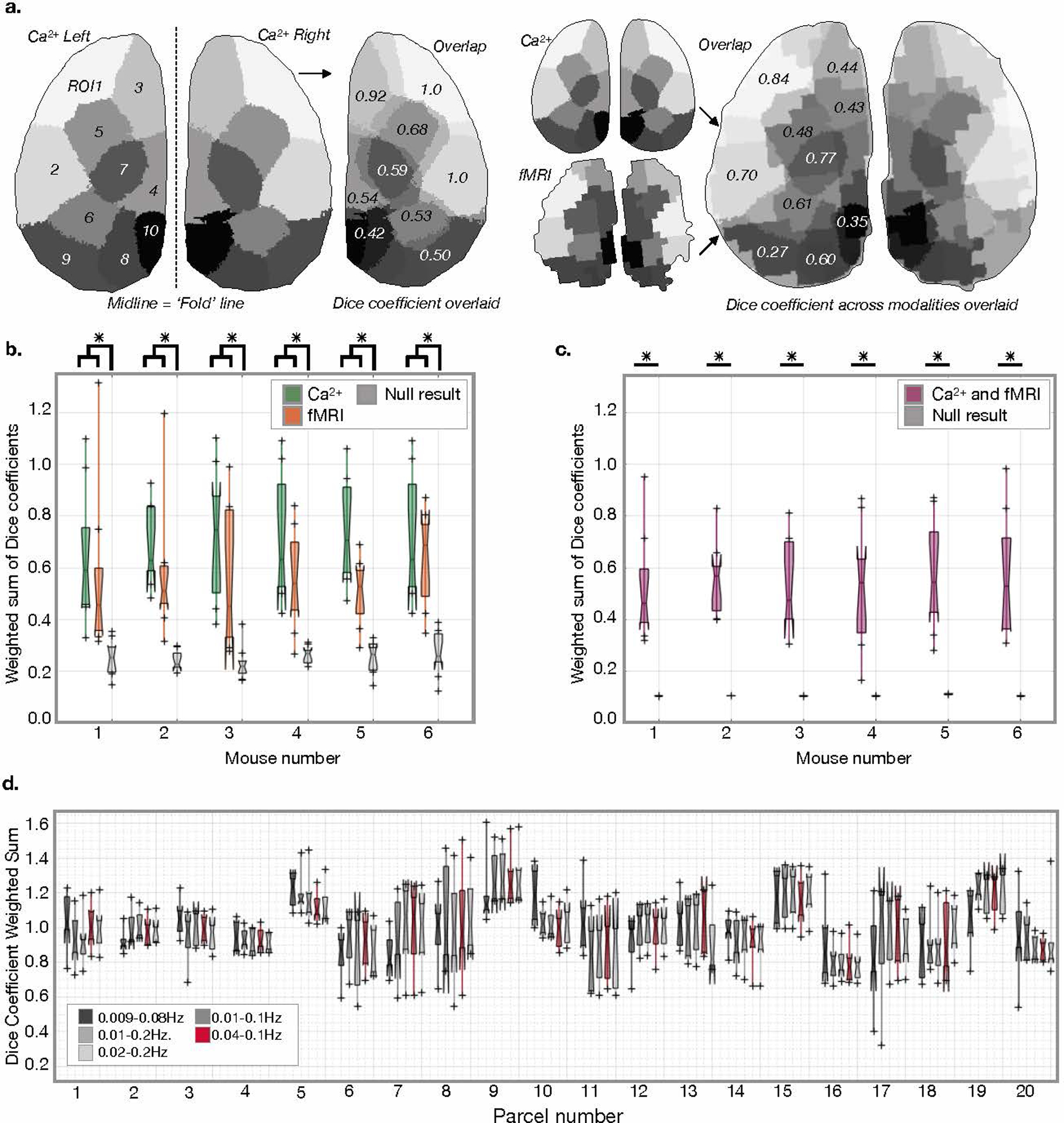
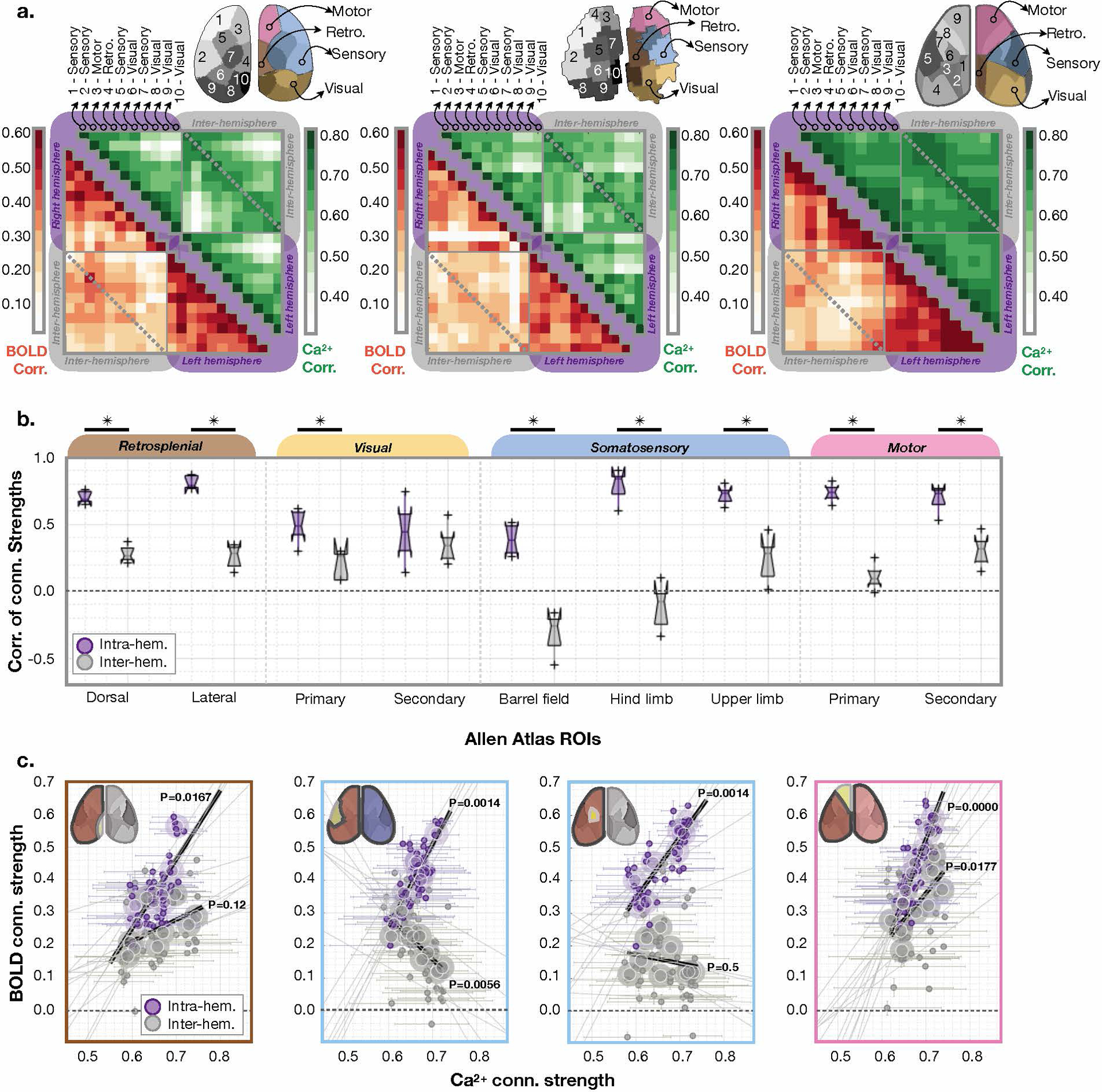
Achieving a comprehensive understanding of brain function requires multiple imaging modalities with complementary strengths. We present an approach for concurrent widefield optical and functional magnetic resonance imaging. By merging these modalities, we can simultaneously acquire whole-brain blood-oxygen-level-dependent (BOLD) and whole-cortex calcium-sensitive fluorescent measures of brain activity. In a transgenic murine model, we show that calcium predicts the BOLD signal, using a model that optimizes a gamma-variant transfer function. We find consistent predictions across the cortex, which are best at low frequency (0.009-0.08 Hz). Furthermore, we show that the relationship between modality connectivity strengths varies by region. Our approach links cell-type-specific optical measurements of activity to the most widely used method for assessing human brain function.

Extended Data Fig. 1. Assembly of MR saddle coil, mouse head-plate, and Ca²⁺ imaging optical apparatus

Custom saddle coil and imaging apparatus design. a) Removable saddle coil, with case that protects hardware. b) Coil in place on dual imaging sled. Coil (white) is mounted on a support system (blue) which is fixed to the sled (semi-transparent blue). A support system for the mouse (orange) is attached to the sled to which the mouse head plate (red) attaches. c) Assembled dual imaging apparatus. The telecentric lens (for Ca²⁺ imaging) is secured above the mouse and saddle coil. The position of the telecentric lens (and housing) can be adjusted (yellow) along the magnet B_o axis to focus the Ca²⁺ image.

Extended Data Fig. 2. A cross section of the optical apparatus

A diagram of the light path overlaid on a cross section of our optical apparatus. The light enters the system via a flexible liquid light guide. At the base of the telecentric lens, the light is bent by 90° degrees to enter the telecentric lens. Upon entering the telecentric lens, the excitation light reflects off of the dichroic mirror and is redirected along the length of the telecentric lens and into the prism at the end of the apparatus. The prism redirects the excitation light onto the mouse cortex. The emission light is similarly re-directed by the prism along the length of the telecentric lens (this time traveling in the opposite direction) and passes through the dichroic mirror. The fiber bundle array is mounted onto the end of the telecentric lens and transmits the light to the room neighboring the magnet where the camera is housed. To focus the Ca²⁺ image, the fiber bundle moves relative to the telecentric lens (red arrows).

Extended Data Fig. 3. Videos of Ca²⁺ data pre- and post-image processing

Representative frames from example videos (Supplementary Video 1 & 2) a) Raw (unprocessed) fluorescence signal (cyan wavelength). A fluorescent bead placed within the dental cement at the right anterior edge of the surgical preparation is indicated (white arrow). The bead is used for right and left identification and motion correction. b) Data from a) after processing. c) Estimated motion parameters based on position of fluorescent bead.

Extended Data Fig. 4. Ray-casting algorithm to create the TOF MR angiogram-projected surface image for multi-modal image registration

a) Three example views of the raw 3D MR angiogram data. Blood vessels have high MR signal intensity. b) Example of a maximum intensity projection (MIP) image (left) and a schematic of our ray-casting approach (right). The MIP is generated following masking which removes signal from anatomy outside of the brain. To show the curvature of the brain surface, and to isolate the blood vessels on the surface of the brain, we use the ray-casting algorithm. We project the MR data along the axis perpendicular to the optical imaging plane. Each pixel is shaded based on brain curvature. c) The resulting 2D projection of the MR image.

Extended Data Fig. 5. Average responses to unilateral hind-paw stimulation

a) Average responses to nine stimuli across N=6 mice. Stimulus onset is denoted by black triangles. Ca²⁺ data (top) and the corresponding fMRI data (bottom) are plotted. The fMRI signal is normalized to the mean. The standard deviation within the responding ROI is shown as shading. b) The average normalized (to peak amplitude), stimulus response across N=6 mice, n=9 stimuli each. This shows the different temporal dynamics of these two modalities. The fMRI signal is delayed, relative to stimulus presentation and the Ca²⁺ signal. c) A zoomed in view of the Ca²⁺ and BOLD signals. Since the Ca²⁺ signal is collected at a relatively high temporal resolution (10Hz), it appears in to be noisy. By zooming in the fast kinetics of these data are shown. No filtering of the Ca²⁺ signal has been applied.

Extended Data Fig. 6. Localization of Ca²⁺ and fMRI responses to stimuli

a) A surface projection of the down-sampled Allen Atlas overlaid on the optical data of an example mouse. The ROI expected to respond to the presented unilateral hind limb stimuli is indicated with a dotted line. b) Responding ROIs from all mice from both modalities normalized to the maximum response amplitude. Calculated as follows if we had two instead of six mice: if voxel (i,j) for mouse #1 on average showed a 40% response relative to the maximum responding voxel for that mouse, and voxel (i,j) for mouse #2 on average showed a 60% response relative to the maximum responding voxel for mouse #2, then voxel (i,j) would be color-coded to 50%. The expected responding ROI from the Allen Atlas is shown as a dotted line. c) An example responding ROI from one mouse overlaid on the optical data. d) The same example responding ROIs (from the same mouse) overlaid on the projected MRI data.

Extended Data Fig. 7. Gamma-variant convolution model applied within responding ROIs identified by GLM

a) Three example 50-second windows from N=3 mice (left and middle panels). Ca²⁺ signal, averaged within the responding ROI, before (green) and after (blue) applying the gamma-variant convolution. BOLD signal (orange), averaged within the responding ROI. The average predicted hemodynamic response function (HRF) from these three examples (right panel). Goodness of fit assessed by correlating (Fisher’s Z transformed Pearson’s correlation) the Ca²⁺ signal convolved with the predicted HRF (blue) and the BOLD signal (orange). b) The correlations for N=6 mice (n=4 session, n=11 windows, i.e. 44 data points per mouse) using filtered [0.04–0.1Hz] (left) or unfiltered (middle) data. Each 50-second window contains the presentation of one unilateral hind-paw stimulus. The Ca²⁺ and BOLD responding ROIs are not fixed across mice, as illustrated (right) [reproduced from Extended Data Fig. 6]. For the boxplots, the central line is the median, the minima and maxima of the box extends to the 25^th and 75^th percentiles, whiskers extend to all data points, and outliers (data points beyond the 25^th to 75^th percentiles) are denoted by ‘+’.

Extended Data Fig. 8. Convolution model applied within Allen Atlas ROIs is not affected by window, frequency band, scan number or mouse

Correlation between Ca²⁺ and BOLD signals. a) Correlation strengths compared across nine scans spanning the duration of our acquisitions. Scans where no stimulus are presented (grey), and during unilateral hind-paw stimulation (green), are different from the null (BOLD time points scrambled). b) Correlation strengths compared across mice. c) Correlation strengths compared between windows. d) Correlation strengths compared within different frequency filters. All show the same relationship to the null using a two-samples t-test. For boxplots, the central line is the median, the minima and maxima of the box extends to the 25^th and 75^th percentiles, whiskers extend to all data points, and outliers (data points beyond the 25^th to 75^th percentiles) are denoted by ‘+’. No correction for multiple comparisons was applied.

Extended Data Fig. 9. Parcellation results are independent of frequency filter across mice and parcel, variance is caused by parcel size

a) Variance across parcels for each mouse for n=5 frequency filters. b) Variance due to parcel for each filter for N=6 mice. Neither frequency filter, nor mouse, captures the variance in the Dice coefficient observed. c) Variance is highly correlated with parcel size. d) Variance across frequency filters for N=6 mice. For the boxplots, the central line is the median, the minima and maxima of the box extends to the 25^th and 75^th percentiles, whiskers extend to all data points, and outliers (data points beyond the 25^th to 75^th percentiles) are denoted by ‘+’.

Extended Data Fig. 10. Inter- vs. intra-hemisphere connectivity strength patterns between Ca2+ and BOLD vary regionally and by brain functional area

a) and b) are reproduced for reference from Figure 6. c) and d) are equivalent plots to b) showing the same information (inter-, purple, and intra-, grey, hemisphere regional connectivity strengths) for the three parcellations shown in a). b) shows results from the Allen atlas, c) shows results from the Ca²⁺ parcellation, and d) shows results from the BOLD parcellation. For the boxplots, the central line is the median, the minima and maxima of the box extends to the 25^th and 75^th percentiles, whiskers extend to all data points, and outliers (data points beyond the 25^th to 75^th percentiles) are denoted by ‘+’.

Fig. 1.. Experimental setup for simultaneous mesoscopic Ca²⁺ and MR imaging.

a) Overview of the components of the imaging set-up, which include an 11.7T, 9cm bore MR scanner, into which we insert the optical components for Ca²⁺ signal acquisition, MRI coil, animal, and physiological monitoring and maintenance equipment. The Ca²⁺ imaging data is recorded by a CCD camera connected to a computer housed in a room adjacent to the scanner. A 4.6m long fiber optic bundle relays the Ca²⁺ signal from within the magnet to the CCD camera. b) Surgical window preparation for acute imaging. The preparation is secured to a plate that cradles the sides of the skull and attaches to the skull above the olfactory bulb. c) Photograph of the assembled dual-imaging apparatus. The plate shown in b) is fixed to the MRI coil below the Ca²⁺ imaging hardware. d) A raw Ca²⁺ image captured using the set-up shown in a) and c). A fiber optic bundle containing ~2 million fibers is used to obtain a FOV spanning the optically exposed FOV.

Fig. 2.. Registration pipeline for simultaneously acquired Ca²⁺ and MRI data.

a) Cartoons depicting the Ca²⁺ (top left) and fMRI (bottom left) acquisitions. Sample MR functional (top right) and structural (bottom right) images. b) Overview of the multi-modal image acquisition and registration pipeline. In addition to the simultaneously acquired Ca²⁺ and fMRI data, we acquire a high in-plane resolution image of the fMRI FOV, an isotropic anatomical MRI of the whole brain, a TOF MR-angiogram, and a high-resolution anatomical image of the tissue within the angiogram FOV. The functional and structural MRI data are registered in ‘individual space’, and then, using non-linear registration, to reference space. c) Steps in the registration pipeline illustrating the use of surface vessels as anatomical landmarks. Left: MR angiogram. Center left: surface projection. Center right: Ca²⁺ image. Right: merged image. Vessels used for registration are indicated in the images.

Fig. 3.. Spontaneous fluctuations of evoked Ca²⁺ and fMRI signals.

a) Evoked responses to unilateral hind-paw stimulation. The average Ca²⁺ (top row) and fMRI (bottom row) responses (to N=9 stimuli) for three example mice are plotted. ROIs were determined using standard generalized linear modeling. The stimulus ON time is denoted by a black line. The fMRI signal is normalized to the mean. The SD across stimulus presentations is shaded. b) Ca²⁺ (top) and fMRI (bottom) ROI data for Mouse #2. c) Average response for Ca²⁺ (top) and fMRI (middle) of an example mouse is plotted over a 10-minute interval encompassing N=9 stimuli. Data are averaged spatially. Yellow: boxcar (top) and HRF (middle) from the GLM models. Bottom: zoomed-in section of the fMRI signal trace. Small (dashed line) and large (solid line) amplitude responses are circled to indicate coincident fluctuations in amplitude. Peak amplitude response estimated by averaging the signal from the peak until three seconds after the peak are shown by black lines at the level of each estimated response amplitude. The normalized response amplitude (relative to the mean signal) is written beneath each response (black triangles denote stimuli onset). d) Correlation for the normalized Ca²⁺ and fMRI response amplitudes in Mouse #3 are z=1.00 P=0.009 (top). Across all 6 mice (n=9 responses per mouse), the correlations are z=0.44, P=0.0023 (bottom). No adjustment was made for multiple comparisons. P-values are from Fisher’s Z transformed Pearson’s correlation, which tests the null hypothesis that a correlation does not exist.

Fig. 4.. Gamma-variate convolution model applied within Allen Atlas ROIs.

a) Average signals within example Allen Atlas regions. Ca²⁺ signal before (green) and after (blue) applying gamma-variate convolution for 50-second windows from N=3 mice. BOLD signal (orange) for the same windows, mice, and atlas regions (left and middle panels). Average predicted HRF across all regions and data for each mouse (right panel). Goodness of fit is assessed by Fisher’s Z transformed Pearson’s correlation between the Ca²⁺ data convolved with the predicted HRF (blue) and the BOLD signal (orange). b) Our down-sampled version of the Allen Atlas. c) Experiment timeline. d) Correlation strength of Ca²⁺ data convolved with the predicted HRF and the BOLD signal for N=6 mice for n=18 Allen Atlas ROIs (n=9 scans, n=11 50-second windows per scan, i.e. 99 data points per mouse). Boxplot terms: central line is the median, the minima and maxima of the box extends to the 25^th and 75^th percentiles, whiskers extend to all data points, and outliers (data points beyond the 25^th to 75^th percentiles) are denoted by ‘+’. No correction for multiple comparisons is applied. We test for a difference between all ROIs and a null distribution (BOLD time points are scrambled) using a two-sample t-test, P=0.0000. Effects of different frequency filters are considered (Extended Data Fig. 8). e) Maps of median estimated gamma variant parameters: amplitude (left), time-of-peak (middle), and width (right).

Fig. 5.. Parcellation using spontaneous Ca²⁺ and fMRI activity.

a) Example of overlap of functional parcellations within (left), and between (right) modalities. To measure the consistency of functional parcellations, we separately parcel the left and right hemispheres for each modality, then compare parcels across hemispheres (left) and modalities (right) using the Dice coefficient. b) Bilateral symmetry of the Ca²⁺ (green), and fMRI (orange) parcellations is above chance (null result from random parcel assignment, gray). For Ca²⁺ data (mouse #1–6): P=0.0001, 0.0000, 0.0000, 0.0000, 0.0000, and 0.0000. For BOLD data (mouse #1–6): P=0.0066, 0.0004, 0.0012, 0.0002, 0.0000, and 0.0000. No correction for multiple comparisons is applied. We test for a difference between Dice coefficients across ROIs using a two-sample t-test. c) Comparison between Ca²⁺ and fMRI parcellations, with parcels overlapping across modalities above chance levels (mouse #1–6): P=0.0000, 0.0000, 0.0000, 0.0000, 0.0000, 0.0000. No correction for multiple comparisons is applied. We test for a difference between Dice coefficients across ROIs using a two-sample t-test. d) Dice coefficients for different parcels, depending on frequency band (Extended Data Fig. 9). For all boxplots the central line is the median, the minima and maxima of the box extends to the 25^th and 75^th percentiles, whiskers extend to all data points, and outliers (data points beyond the 25^th to 75^th percentiles) are denoted by ‘+’.

Fig. 6.. Inter- vs. intra-hemisphere connectivity strength patterns between Ca²⁺ and BOLD vary regionally and by brain function.

a) Ca²⁺ (left), BOLD (middle), and Allen Atlas (right) connectivity matrices averaged across mice (N=6). ROIs within the Ca²⁺ and BOLD parcellations are labeled based on proximity to regions defined by the Allen Atlas, with the exception of the somatosensory lower limb area which can be identified by evoked responses. b) Correlation between the Ca²⁺ and BOLD connectivity strengths for each region both intra- (purple) and inter-hemisphere (grey) for Allen atlas regions. We test for a difference between inter- and intra-hemisphere connectivity across ROIs using a two-sample t-test (left to right): dorsal P=0.0000, lateral P=0.0000, primary visual P=0.0042, secondary visual P=0.4317, barrel field P=0.0000, hind-limb P=0.0000, upper-limb P=0.0003, primary motor P=0.0000, secondary motor P=0.0005. For the boxplot, the central line is the median, the minima and maxima of the box extends to the 25^th and 75^th percentiles, whiskers extend to all data points, and outliers (data points beyond the 25^th to 75^th percentiles) are denoted by ‘+’. c) The correlation of the Ca²⁺ and BOLD connectivity strengths show different relationships across functional regions within and between hemispheres. Four example regions are shown (left to right): dorsal (left), barrel (left middle), hind limb (right middle), and motor (right). No adjustment is made for multiple comparisons. P-values are from a two-sided test (obtained using Fisher’s Z transformed Pearson’s correlation) which tests the null hypothesis that a correlation does not exist. Data from each edge is averaged across mice (small circles) and across scans (large circles).

References

1. Ross WN. Understanding calcium waves and sparks in central neurons. Nat Rev Neurosci 13, 157–168 (2012). - PMC - PubMed
1. Barson D et al. Simultaneous mesoscopic and two-photon imaging of neuronal activity in cortical circuits. Nat Methods 17, 107–113 (2020). - PMC - PubMed
1. Ogawa S et al. Brain magnetic resonance imaging with contrast dependent on blood oxygenation. Proc Natl Acad Sci USA, 87, 9868–9872 (1990). - PMC - PubMed
1. Albers F et al. Multimodal functional neuroimaging by simultaneous BOLD fMRI and fiber-optic calcium recordings and optogenetic control. Mol Imaging Biol, 20, 171–182 (2018). - PubMed
1. Hyder F et al. Neurovascular and neurometabolic couplings in dynamic calibrated fMRI: Transient oxidative neuroenergetics for block-design and event-related paradigms. Front Neuroenerg, 2, 1–11 (2019). - PMC - PubMed
Publication types