Blind Resolution of Lifetime Components in Individual Pixels of Fluorescence Lifetime Images Using the Phasor Approach

Abstract

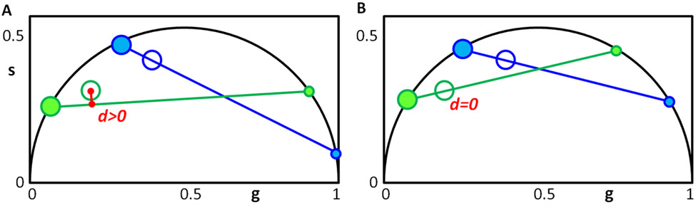
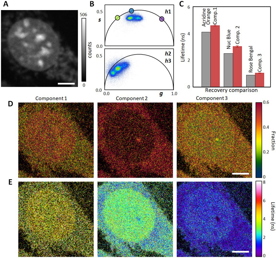
The phasor approach is used in fluorescence lifetime imaging microscopy for several purposes, notably to calculate the metabolic index of single cells and tissues. An important feature of the phasor approach is that it is a fit-free method allowing immediate and easy to interpret analysis of images. In a recent paper, we showed that three or four intensity fractions of exponential components can be resolved in each pixel of an image by the phasor approach using simple algebra, provided the component phasors are known. This method only makes use of the rule of linear combination of phasors rather than fits. Without prior knowledge of the components and their single exponential decay times, resolution of components and fractions is much more challenging. Blind decomposition has been carried out only for cuvette experiments wherein the statistics in terms of the number of photons collected is very good. In this paper, we show that using the phasor approach and measurements of the decay at phasor harmonics 2 and 3, available using modern electronics, we could resolve the decay in each pixel of an image in live cells or mice liver tissues with two or more exponential components without prior knowledge of the values of the components. In this paper, blind decomposition is achieved using a graphical method for two components and a minimization method for three components. This specific use of the phasor approach to resolve multicomponents in a pixel enables applications where multiplexing species with different lifetimes and potentially different spectra can provide a different type of super-resolved image content.

Figure 1.. Graphically finding two unknown lifetime components and their relative fractional intensities.

A) The universal circle is scanned for candidate components. For each position of the first component (small blue dot), a line is drawn through the data point (blue empty circle) and a second point is found where the blue line meets the universal circle (large blue filled circle). The second harmonic (h2) for the candidate components are obtained mathematically: (small green dot) and the large green filled circle. A line is drawn through them (green line). B) The solution is the only lifetime pair that has the lines (blue and green) going through the data points for the two harmonics, i.e. when the distance from the green line to the green empty circle is zero. The relative fractions are obtained by the ratios between the distances from the filled dots to the empty circles in both sides of the line.

Figure 2.. Finding the 3 lifetime components in the universal circle.

A) Schematic configuration of 3 components generating a data point (ring in the middle). As an example, the ratio between the two distances is related to the intensity fraction of the component located in the short lifetime region; $f_1=d_1∕(d_1+{\tilde{d}}_1)$. In the same manner the other two fractions can be obtained for the other two components. B) The solution to the 3 component problem is the only combination of components such that the three fractions are the same in each of the triangles composed by the three harmonics (blue-green-orange). The short, medium and long lifetime components in each harmonics are depicted by increasingly larger filled circles.

Figure 3.. Simulations for 2 components, one fixed one variable.

The points in the graphs are the recovered lifetimes. A) Lifetime component of 4 ns (black) (right) is mixed in the same pixel in equal fractional intensity with a variable lifetime component (red) that spans the range from 0 to 8 ns. When the two lifetime components become similar (simulation measurements from 40 to 50), the algorithm shows a lifetime component at around 4 ns and another component whose value and fraction is undefined, as it should, since in this range there is effectively only one lifetime. B) We fixed the fractional intensity of the first component to have the same value for all the simulation. In this case the two lifetime values are recovered perfectly even if they are very close to one another.

Figure 4.. Simulation for blind recovery of 3 components and 3 intensity fractions.

The points in the graphs are the recovered components. A) One lifetime component simulated was 8 ns (black), another was 4 ns (blue) and a third lifetime component was added with variable lifetime (red) from 0.02 ns to 2.0 ns in steps of 0.02 ns. The fractional intensities were 0.5, 0.3 and 0.2, for the 3 components, respectively. Panel A shows that this system can be recovered exactly in the simulations because the lifetimes are different in all the range of the simulation. B) Recovery of the 3 components when two lifetimes become very close. The lifetime set was 8 ns (black), 1 ns (blue) and a variable lifetime from 0.02 ns to 4 ns (red). As this variable component lifetime increases, the recovered value of the 8 ns component changes from around 8ns, reaching a maximum of about 9 ns when the variable component is similar to the second components at 1 ns. As the variable component continues to increase in lifetime value, it causes a decrease of the long lifetime returning to 8 ns and a stabilization of the 1ns component when the added component reaches a value of 2 ns or longer. This simulation shows that the blind independent determination of 3 components is difficult because one component can influence the others when two of the components have similar lifetimes. C) However, if we fix the relative contribution of the long components to the value of 0.5 we get a perfect recovery of the 3 lifetimes. This simulation demonstrates that the lifetimes and fractions are correlated. If we fix the fraction of one component, then the systems can be recovered exactly.

Figure 5.. Effect of noise on the recovery of components.

The points in the graph are the recovered lifetimes A) Simulation of 3 lifetime components, no noise added. Black, Blue and Red represent 8, 4, 1 ns lifetimes in each individual measurement/simulation. B) Noise is added only to the 8ns component. Note that the other components lifetimes are not affected by the noise added to the 8ns component. C) Noise is added to the harmonics (not lifetime) of the 8 ns component. Here we show that other components (4 ns/ 1ns) get affected when the noise is added to the harmonics.

Figure 6.. Results of measurements with prepared dye solutions.

The expected (grey) and the recovered (red) components are shown next to each other in each case. A) Recovery in the preparations containing two mixed dyes. C) Recovery in the combinations of three mixed dyes. D) Recovery in the preparation with four mixed dyes. In each case the component id numbers correspond respectively to: 1-Dansyl acid, 2-Fluorescein, 3-Eosin Y and 4-Sulfo-Cy3. The errors in the red bars are the pixel-wise standard deviation of the recovered data. B) For each pair combination, the difference in lifetime between the two components is plotted with the standard deviation in the recovery of the longest of the couple, showing a clear dependency. In each case, the decreasing difference between the long and short lifetime increases the width of the distribution of the recovered long lifetime and the distribution width depends on the value of long lifetime. In the single combination of the four component system (D) we repeated the experiment by fixing the long lifetime to the known value of 11.8 ns (right side of panel D) which substantially improves the recovery of the lifetime components.

Figure 7.. Three-component blind recovery in live cells.

Representative FLIM experiment of a cell with the addition of nuclear dyes (Acridine Orange, Nuc Blue and Rose Bengal). A) Intensity image, scale bar 5μm. In this example we have a large number of counts in the bright dots in the nucleus (scale bar at the right of the panel). B) Smoothed phasor plots for the first harmonic (h1) and the second and third harmonic together (h2, h3). The colored circles on the universal circle indicate the measured phasor position of the first harmonic of the individually-measured dyes in cells; Acridine Orange (green), Nuc Blue (blue) and Rose Bengal (purple). C) Bar plot comparing lifetime measurements of the individual dyes measured independently (grey) and recovered from the algorithm (red) using 3 blind components. Errors show the standard deviation of the recovered values in three cells. After recovering lifetimes and fractions for 3 components at each pixel, images are reconstructed (color-coded) with the recovered values for fractions (D) and lifetimes (E) according to the color scales on the right.

Figure 8.. Three-component blind recovery in liver tissue samples allows studying metabolic changes.

A) Representative zoom-in intensity images (optical zoom = 40x) of liver slices of mice fed with low-fat (LF) or western diet (WD) are shown (intensity scale bar at the right of the panel). Scale bar 40μm. High counts are observed in the fat droplets in the liver. B) Recovered lifetimes from the algorithm using 3 blind components are represented as violin plots (gray) and the median ± standard deviation. Expected lifetime values for individual species reported in the literature are shown with a horizontal dotted line (red). C) The colored circles on the universal circle indicate the recovered first harmonic phasor position of free NADH (cyan), protein bound NADH (purple) and long-lifetime species (LLS, yellow). D) Fractional intensity distributions of the three components in whole tissue samples (LF and WD) imposing the recovered median lifetimes (also depicting median ± standard deviation). Bound NADH vs free NADH fractional intensity ratios are shown in red (by excluding LLS). E) Color coded phasor-FLIM images of the whole tissue sections of LF (left) and WD (right) mice model (optical zoom= 10x). The free-to-bound ratio (excluding LLS) is color coded using a magenta to cyan colormap with a yellow overlay for LLS above 75%. Scale bar is 1 mm. The bright circle in in the LF sample (row 3, column 5) is due to an air bubble.

References

1. Digman MA; Caiolfa VR; Zamai M; Gratton E, The Phasor Approach to Fluorescence Lifetime Imaging Analysis. Biophys J 2008, 94 (2), L14–L16. - PMC - PubMed
1. Niesner R; Peker B; Schlüsche P; Gericke K-H, Noniterative Biexponential Fluorescence Lifetime Imaging in the Investigation of Cellular Metabolism by Means of NAD(P)H Autofluorescence. Chemphyschem 2004, 5 (8), 1141–1149. - PubMed
1. Ranjit S; Malacrida L; Jameson DM; Gratton E, Fit-free analysis of fluorescence lifetime imaging data using the phasor approach. Nat Protoc 2018, 13 (9), 1979–2004. - PubMed
1. Clayton AHA; Hanley QS; Verveer PJ, Graphical representation and multicomponent analysis of single-frequency fluorescence lifetime imaging microscopy data. J Microsc 2004, 213 (1), 1–5. - PubMed
1. Jameson DM; Gratton E; Hall RD, The Measurement and Analysis of Heterogeneous Emissions by Multifrequency Phase and Modulation Fluorometry. Appl Spectrosc Rev 1984, 20 (1), 55–106. - PubMed
Publication types