Host variables confound gut microbiota studies of human disease

Abstract

Low concordance between studies that examine the role of microbiota in human diseases is a pervasive challenge that limits the capacity to identify causal relationships between host-associated microorganisms and pathology. The risk of obtaining false positives is exacerbated by wide interindividual heterogeneity in microbiota composition¹, probably due to population-wide differences in human lifestyle and physiological variables² that exert differential effects on the microbiota. Here we infer the greatest, generalized sources of heterogeneity in human gut microbiota profiles and also identify human lifestyle and physiological characteristics that, if not evenly matched between cases and controls, confound microbiota analyses to produce spurious microbial associations with human diseases. We identify alcohol consumption frequency and bowel movement quality as unexpectedly strong sources of gut microbiota variance that differ in distribution between healthy participants and participants with a disease and that can confound study designs. We demonstrate that for numerous prevalent, high-burden human diseases, matching cases and controls for confounding variables reduces observed differences in the microbiota and the incidence of spurious associations. On this basis, we present a list of host variables that we recommend should be captured in human microbiota studies for the purpose of matching comparison groups, which we anticipate will increase robustness and reproducibility in resolving the members of the gut microbiota that are truly associated with human disease.

Extended Data Figure 1:. Data processing and machine learning analysis framework.

Raw V4 16S rRNA reads were processed using dada2 and samples were filtered and selected as described in the text and Methods to form the ‘core sample population’. Balanced cohorts were constructed for each binary questionnaire variable, and Random Forests analyses were repeated 25 times over 75/25 splits. Concurrently, sample classes were randomly permuted to simulate noise and the same procedure was performed to facilitate empirical P value estimations.

Extended Data Figure 2:. Machine learning evaluation of common exclusion criteria and variables for matching.

A) Random Forests analysis was performed on binary metadata variables commonly used to shape comparative gut microbiota surveys (N=4,038 subjects). Red labels represent variables chosen for exclusion while blue labels represent included subjects. Center lines represent median values of 100-repeat mean AUROC’s, boxes denote interquartile ranges, and whiskers denote 1.5*interquartile ranges. B) Support vector machine analysis was performed on subjects by age group. Shown is a normalized confusion matrix, averaged across all cross-validation folds. Hierarchical clustering using Euclidean distances with average weighting is shown to the right. C) Random Forests AUROC values for all variables with empirical P < 0.05, shown by variable category. Analysis results for “disease-inclusive” cohorts (with only T2D and IBD removed as per final exclusion criteria, N=5,878) are shown as well as results using only subjects reporting no medical diagnoses of diseases (“disease-exclusive” cohorts, N=2,971). Center lines represent median values of 100-repeat mean AUROC’s, boxes denote interquartile ranges, and whiskers denote 1.5*interquartile ranges. D) Random Forests AUROC values for physiological, lifestyle, and diet variables in subjects reporting no medical diagnoses of diseases (“disease-exclusive” cohorts, N=2,971; x-axis) compared to disease-inclusive cohorts (N=5,878). Outlined in black are representative cohorts for all variables chosen for matching. For frequency-based variables, the frequency categories (e.g. daily, regular) with highest AUROC in the disease-exclusive cohorts are outlined. E) Spearman co-correlation heatmap of all top microbiota-associated variables (those with median AUROC > 0.7 and P < 0.05 by Random Forests). Absolute values of Spearman rho correlation coefficients are shown for each variable pair at their intersections. F) Whole grain consumption frequency between non-celiac subjects reporting no dietary gluten intake (a binary variable that exhibited mean AUROC > 0.7 and P < 0.05 by Random Forests). G) Whole grain consumption frequency between celiac subjects and non-celiac subjects that report no special gluten-free diet (also mean AUROC > 0.7 and P < 0.05). H) Subjects taking vitamin supplements are older than those not taking vitamin supplements. As in F and G, significance assessed by two-sided Mann-Whitney U test. I) Age and smoking frequency display a non-monotonic association. Accordingly, ‘Hoeffding’s D’ statistical test was used to find a significant non-monotonic association between the two variables.

Extended Data Figure 3:. Evaluation of Random Forest microbiota association strengths compared to beta diversity assessments and as a function of sample size.

Shown are plots wherein each dot represents results for a single binary cohort representing a single variable including all those listed in Supplementary Table 1. Cohort sizes were capped at 1,500 cases and controls. P values and non-parametric Spearman correlation coefficients are shown in each plot for each comparison. A) Random Forest AUROC values correlate with beta diversity-based PERMANOVA F statistics, and finds significant differences between cases and controls for fewer cohorts than does PERMANOVA. B) Sample size exhibits no significant correlation with Random Forests AUROC values. C) Sample size correlates with PERMANOVA F statistics. D) Sample size correlates strongly with PERMANOVA R² effect size values for each variable. E) From binary and frequency host variables, variables were selected that had n>800 samples and mean AUROC>0.65 (total N=21 host variables). Sample cohorts for each variable were systematically down-sampled by random selection of subjects such that one case-control cohort was constructed with n=50, 100, 150, 200, and then in size increments of 100 until reaching the final cohort size. Mean AUROC values were calculated for each cohort and mean values are represented by red dots with blue depicting 95% confidence interval. F) Cohort size for maximal model accuracy was determined as the first cohort size at which Random Forests empirical P reached a value less than 0.05 and mean AUROC reached a 90% interval of the final AUROC (that of the full cohort).

Extended Data Figure 4:. Comparison of microbiota-host variable association strengths between disease-inclusive and disease-exclusive cohorts.

A-B) Differences in PERMANOVA F statistics between matched and unmatched cohorts within disease-exclusive analyses with all subjects reporting medical diagnoses removed, analogous to Figure 2. Subjects in ‘matched’ cohorts were matched for confounding variables shown to differ between cases and controls (purple) in panel A on a per-disease basis. Boxes represent interquartile ranges in F statistics from 25 permuted cohorts per matched/unmatched condition. Center lines within boxes represent median F statistic values. C) F statistics denoting differences between cases and controls for each disease among unmatched (location-only matched) cohorts comparing disease-exclusive to disease-inclusive results. Spearman rho= 0.81, P = 3.2*10⁻⁵. D) F statistics denoting differences between cases and controls for each disease among confounder-matched cohorts comparing disease-exclusive to disease-inclusive results. Spearman rho= 0.64, P = 2.9*10⁻³. E) Concordance in whether matching reduces or increases case-control microbiota differences were examined for disease-inclusive and disease-exclusive results. Differences in F statistics between matched and unmatched cohorts for each disease were calculated. Shown are F statistics differences for disease-inclusive cohorts (x-axis) and disease-exclusive cohorts (y-axis). Chi-square P = 0.0073, assuming random distribution of points across quadrants as the null hypothesis.

Extended Data Figure 5:. Machine learning and compositional analyses for diseases before and after confounder matching.

A) Matching cases and controls for key microbiota confounding variables substantially reduces observed microbiota differences between cases and controls, as assessed by machine learning methods. Random Forests analysis was performed as in Figure 2 on location-paired unmatched case control cohorts (red boxes) and case control cohorts matched for confounding variables shown in Figure 2 (blue boxes). Empirical P value significance based on comparison of AUROCs to permuted ‘shuffled’ data was calculated as described in methods. Boxes represent interquartile ranges in 100-repeat mean AUROC values per matched/unmatched condition. Center lines within boxes represent median AUROC values. B) Numbers of differentially abundant ASVs in disease cases versus controls before and after matching cohorts for confounding variables. ANCOM W score thresholds were calculated and ASVs are shown that met each threshold. Notably for type 2 diabetes, 26 ASVs differed significantly before matching, while zero ASVs differed post-matching.

Extended Data Figure 6:. Assessment of capacity for statistical methods to correct for mis-matching.

Linear mixed effects analyses were performed as described for Figure 4J. A) Shown are ASVs that passed unadjusted P < 0.05 in the comparison of diabetics to non-diabetic controls via linear mixed effects models, as compared to the more conservative cutoffs shown in Figure 4J (Benjamini-Hochberg Q value < 0.05). B) Shown are ASVs with Benjamini-Hochberg Q value < 0.05 in the comparison of diabetics to non-diabetic controls via linear mixed effects models, with ASVs associated with confounding variables identified by ANCOM as having a W score indicating rejection of the null hypothesis for >80% of log ratio comparisons for that ASV.

Extended Data Figure 7:. Validation of confounding effects of host variables in external independent cohorts of type 2 diabetes and metabolic syndrome.

A) Microbiota-associated host variable distributions between cases and controls in prominent type 2 diabetes gut microbiota surveys. Unpaired t-tests were performed where raw data was available. For studies in which raw data was partial or not found, P values reported in each original publication are shown (Forslund et al., Egshatyan et al.). Center lines denote mean and whiskers denote standard deviation. B) Matched and unmatched T2D case-control cohorts were constructed from independent studies shown. Student’s T test was used to compare PERMANOVA F statistic values between randomly selected unmatched cohorts to cohorts that were matched for available confounder metadata (age, BMI, and BMI respectively). Cohort selections were bootstrapped by re-selecting case and control subjects 25 times for both unmatched and matched cohorts. Metformin+T2D were selected for comparison to non-diabetic controls for the study by Forslund et al. Success of matching was assessed using Wilcoxon signed-rank tests and matched cohorts exhibited median Q>0.05 (ns) for each available confounding variable. C) Metabolic syndrome was examined in an external independent study. BMI, age, and sex were found to differ between location-matched (matched by district in Guangdong) subjects and metabolic syndrome cases. Subjects were matched by these variables including district, and F statistics were compared to unmatched (district-only-matched) case-control cohorts. Center lines represent median values, boxes denote interquartile ranges, and whiskers denote 1.5*interquartile ranges. * P ≤ 0.05; ** P ≤ 0.01; *** P ≤ 0.001; **** P ≤ 0.0001

Extended Data Figure 8:. Assessment of strength of confounding effects for microbiota-associated confounding host variables.

A) Cases and controls were matched for all relevant matching variables except one that was held out (‘leave one out’ [LOO]). The impact of the single variable held out was then assessed by comparing the increase of PERMANOVA F statistic between cases and controls to that of the total change in F statistic from fully matched to unmatched case-control cohorts. Thus, an assessment for the relative independent contribution of each variable to confounding effects in the setting of matching for all other variables was obtained for each variable for each disease. B) Matching by a single variable was performed and resulting F statistics were similarly compared to the difference in F statistics from unmatched to fully matched cohorts, as described in Methods. In A and B, center lines represent median values, boxes denote interquartile ranges, and whiskers denote 1.5*interquartile ranges.

Extended Data Figure 9:. Examination of effects of alcohol consumption on the gut microbiota with external validation.

A) ASV abundances were collapsed to the genus level and log₁₀ mean fold changes were calculated between daily versus never drinkers in the AGP dataset (x axis) and compared to log₁₀ mean fold changes in daily/weekly versus monthly/never drinkers in an external validation dataset (y axis). Spearman correlation test P = 10⁻⁴ B) ASVs in differential abundance in all alcohol consumer cohorts compared to matched control non-drinker subjects, by ANCOM. Matched cohorts were constructed by selecting controls matched for all confounding variables and ANCOM was performed. ASVs found to differ significantly between cases and controls are marked by green circles and denoted by their ANCOM threshold. C) Alcohol consumption frequency, number per session, and cumulative weekly consumption are confounded for various microbiota-associated host variables. D) Microbiota covariate association strength as estimated by Random Forests empirical P value tests for alcohol consumption cohorts. Alcohol subjects were matched to never-drinker controls for confounding variables shown in Extended Data Figure 9A and Random Forests analysis was performed as in Figure 2. Bars denote interquartile ranges of AUROCs from 100 repeats. Empirical P=0.0739, P=0.0495. E) Subjects reporting drinking only one type of alcohol (beer/cider, red wine, white wine, or spirits/hard alcohol), were compared to non-drinkers matched for variables shown in (C). Cohort sample sizes were increased when including drinkers who consumed multiple types, and significant median PERMANOVA P values were observed: P=0.004, P=0.007, P=0.021, P=0.076. In D and E, center lines represent median values, boxes denote interquartile ranges, and whiskers denote 1.5*interquartile ranges. F) Alpha diversity was calculated for subjects reporting consumption of each alcohol type (inclusive of those who also drink other types). Lines depict differences in median alpha diversity between cases and controls for each of the 25 re-sampled case-control cohorts. Unadjusted two-sided paired Student’s t-tests were performed. † P ≤ 0.10, *P ≤ 0.05.

Extended Data Figure 10:. Bowel movement quality matching and external validation.

A) Subjects reporting solid or loose bowel movement (BM) quality were compared to subjects reporting normal BM quality in terms of their distribution of microbiota-confouding variables. All BM subject cohorts were thus subsequently matched for sex, alcohol, BMI, whole grain, and salted snack consumption (for Figure 4E–F). B) ASV abundances were collapsed to the genus level and log₁₀ mean fold changes were calculated between solid versus normal BM quality subjects AGP dataset (x axis) and compared to log₁₀ mean fold changes in sold versus normal BM quality subjects in an external validation dataset (y axis). Spearman correlation test P = 10⁻¹⁶

Figure 1:. Physiological, lifestyle, and dietary characteristics strongly associate with gut microbiota composition.

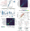
A) Random Forests analysis results for binary physiological, lifestyle, and diet variables. All variables shown exhibited P < 0.05 by empirical P value permutation tests. Blue labels are proposed as matching variables for examination in subsequent analyses (those of Figure 2 and beyond). B) Random Forests analysis results for frequency-based lifestyle and dietary intake variables. For each frequency category (i.e. ‘daily’, ‘regular’, ‘occasional’, and ‘rare’), binary cohorts were constructed with control subjects comprising those who self-reported ‘never’ for that variable. Frequency categories for each variable exhibiting P < 0.05 are denoted by dots over bars for frequency variables. In A and B, solid bars denote means, boxes denote upper inter-quartile ranges, and whiskers denote standard deviation of AUROC values from 100 repeats of Random Forests classifiers.

Figure 2:. Human disease subjects vary from healthy controls in critical microbiota-associated variables that confound microbiota analyses.

A) Shown in purple are variables that differ in disease cases versus randomly selected location-paired control subjects (Benjamini-Hochberg Q value < 0.05). For continuous variable comparisons (age, BMI) a two-sided Mann-Whitney U test was performed, while for remaining categorical variable comparisons a Fisher’s exact test was performed. B) Shown are differences between beta diversity-based F statistics of unmatched, location-paired disease case-control cohorts and those of fully matched case-control cohorts. Analyses were augmented using a bootstrapping control cohort re-selection method to assess dispersion of microbiota community differences (described in Methods). Red boxes represent interquartile ranges in F statistics from 25 randomly selected location-paired unmatched cohorts, while blue boxes represent interquartile ranges in F statistic from 25 randomly selected cohorts for which controls were selected that matched cases for all microbiota-associated host variables that differed between cases and controls shown in (A). Center lines within boxes represent median F statistic values.

Figure 3:. Microbiota variation due to confounding variables spuriously increases observations of disease-associated microbiota differences.

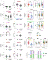
(A-C) Differences between type 2 diabetes subjects and non-diabetic control subjects (N=126) for alcohol frequency (Benjamini-Hochberg [BH] Q=0.0015, Fisher’s exact test) (A), BMI (BH Q=4.14*10⁻⁹, two-sided Mann-Whitney U test) (B), and age (BH Q=5.94*10⁻⁵, two-sided Mann-Whitney U test) (C). D) Principal coordinates analysis (PCoA) plot of diabetes cases and control subjects unmatched for aforementioned variables, with median PERMANOVA P value and F statistics shown. Subject group centroids are depicted by an outlined circle. (E-G) Differences between type 2 diabetes subjects and fully matched non-diabetic control subjects for alcohol frequency (E), BMI (F), and age (G). H) PCoA plot of confounder-matched diabetes cases and controls. I) Random Forest AUROC values for diabetes cases and controls before and after matching for confounding variables. J) Linear mixed effects models were constructed as described in Methods to include age, BMI, and alcohol intake frequency as confounding covariates. Shown are ASVs that passed BH Q values < 0.05 cutoffs for each analysis. Boxes denote inter-quartile range, black bar denotes median, and whiskers denote range.

Figure 4:. Alcohol intake and bowel movement quality are associated with robust effects on microbiota composition that confound microbiota studies of human disease.

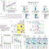
A) Case/control cohorts for type 2 diabetes were constructed by matching for no host variables (‘Unmatched’), matching for all three discordant variables together (‘Fully Matched’), and matching for either each variable individually or all variables but one in a leave-one-out (LOO) analysis (with the left-out variable indicated after ‘LOO’). Microbiota association estimates were quantified using beta diversity-based F statistics as described in the text. Significance of differences in F statistics was assessed by two-sided Student’s t-test. P=0.002, P=2.7*10⁻¹¹. B) Shannon diversity by alcohol frequency categories. Thick black bars represent median values, boxes delineate quartile values. Spearman P=4.8*10⁻¹⁴. C) Alcohol subjects were matched to non-drinker controls for confounding variables (Extended Data Figure 9C) and bootstrapped beta diversity F statistics were calculated. Median PERMANOVA P values are shown. P=0.021, P=0.011, P=0.006; P=0.018, P=0.01, P=0.016; P=0.004, P=0.004. D) Cohorts were constructed as in (A) by matching by one variable individually or LOO analyses as indicated. P=1*10⁻¹⁰. E) Single-variable matching and LOO cohorts were similarly constructed for ASD. P= 0.004, P=8*10⁻⁵. F) Canberra-based PCoA ordinations depicting solid, normal, and loose bowel movement quality (BMQ) subjects (Bristol stool scores 1–2, 3–4, and 5–7, respectively). Group centroids are depicted by large dark-outlined circles. Inter-group PERMANOVA P = 1*10⁻⁵. G) BMQ subjects were matched to controls for confounding variables (Extended Data Figure 10A) and bootstrapped beta diversity F statistics were calculated. Boxes denote inter-quartile range, black bar denotes median, and whiskers denote range. Median PERMANOVA P values are shown. P=0.0003, P=0.006. * P < 0.05; ** P < 0.005; *** P < 0.0005.

References

1. Huttenhower C et al. Structure, function and diversity of the healthy human microbiome. Nature (2012) doi:10.1038/nature11234. - DOI - PMC - PubMed
1. Falony G et al. Population-level analysis of gut microbiome variation. Science (80-. ). (2016) doi:10.1126/science.aad3503. - DOI - PubMed
1. Hsiao EY et al. Microbiota modulate behavioral and physiological abnormalities associated with neurodevelopmental disorders. Cell (2013) doi:10.1016/j.cell.2013.11.024. - DOI - PMC - PubMed
1. Plovier H et al. A purified membrane protein from Akkermansia muciniphila or the pasteurized bacterium improves metabolism in obese and diabetic mice. Nat. Med (2017) doi:10.1038/nm.4236. - DOI - PubMed
1. Belkaid Y & Hand TW Role of the microbiota in immunity and inflammation. Cell (2014) doi:10.1016/j.cell.2014.03.011. - DOI - PMC - PubMed
Publication types