Graph Search-Based Exploration Method Using a Frontier-Graph Structure for Mobile Robots

Abstract

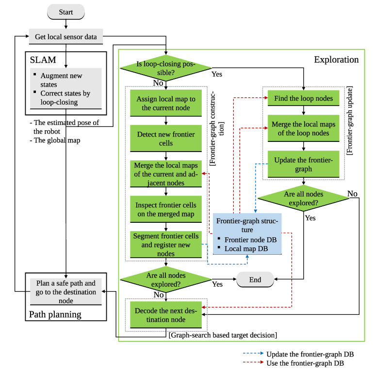
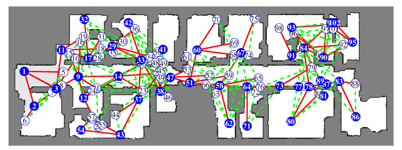
This paper describes a graph search-based exploration method. Segmented frontier nodes and their relative transformations constitute a frontier-graph structure. Frontier detection and segmentation are performed using local grid maps of adjacent nodes. The proposed frontier-graph structure can systematically manage local information according to the exploration state and overcome the problem caused by updating a single global grid map. The robot selects the next target using breadth-first search (BFS) exploration of the frontier-graph. The BFS exploration is improved to generate an efficient loop-closing sequence between adjacent nodes. We verify that our BFS-based exploration method can gradually extend the frontier-graph structure and efficiently map the entire environment, regardless of the starting position.

Keywords: breadth-first search; depth-first search; exploration; frontier detection; loop-closing; mobile robots.

Figure 1

Overview of the proposed integrated exploration algorithm using a frontier-graph structure and graph search-based decision.

Figure 2

Examples of frontier segmentation. Medium gray indicates unknown cells; black indicates occupied cells; very light gray indicates empty cells; red stars are detected frontier cells; cyan dots are representative nodes; red dots are current nodes; yellow dots are unexplored next targets; the blue dot is the next explored target; cyan lines show the solution to the traveling salesman problem (TSP) for the current node and its child nodes: (a) Local map constructed at the root node (b) local map constructed at the root node’s first child node (c) local map constructed at the root node’s third child node (d). A single map is used at the root node to discriminate real frontiers. (e) The local maps of the current and parent nodes are merged. The previous node is the parent node. The root/parent node’s second child node is not at the frontier area in the merged map, and is eliminated from the exploration target list to obtain a new observation. (f) The local maps of the current, parent, and previous nodes are merged. The previous node is the sibling node.

Figure 3

Frontier cell detection: (a) Local grid map. (b) Empty region of local grid map. (c) Internal boundary of empty region extracted by morphological operations. (d) Safe frontier cells (red stars) on merged map.

Figure 4

Registering the edges between the current and revisited nodes’ neighbors in the frontier node DB after accidental loop-closing.

Figure 5

The environment and 80 starting positions.

Figure 6

Simulation results. Maximum range of the LRF is 4 m: (a) Number of exploration steps until the exploration is completed. (b) Total number of registered frontier nodes in the frontier-graph. (c) Number of active nodes. (d) Total traveling distance.

Figure 7

Simulation results. Maximum range of the LRF is 8 m: (a) Number of exploration steps until completion of exploration. (b) Total number of registered frontier nodes in the frontier-graph. (c) Number of active nodes. (d) Total traveling distance.

Figure 8

Resulting frontier-graph structure on the final grid map by the BFS exploration. The number is the ID of each frontier node. Red lines are edges between the parent and child nodes. Dotted green lines are edges between sibling nodes. Blue circles are active nodes, and white circles are inactive nodes: (a) Frontier-graph from 4 m LRF. (b) Frontier-graph from 8 m LRF.

Figure 9

Frontier-graph structure on the final grid map obtained from BFS exploration. The numbers indicate the ID of each frontier node. Red lines are edges between the parent and child nodes. Dotted green lines are edges between sibling nodes. Blue circles are active nodes, and white circles are inactive nodes.

References

-
- Latif Y., Cadena C., Neira J. Robust loop closing over time for pose graph SLAM. Int. J. Robot. Res. 2013;32:1611–1626. doi: 10.1177/0278364913498910. - DOI
- Yamauchi B. Frontier-based exploration using multiple robots; Proceedings of the Second International Conference on Autonomous Agents; Minneapolis, MN, USA. 9–13 May 1998; pp. 47–53.
- Shade R., Newman P. Choosing where to go: Complete 3D exploration with stereo; Proceedings of the 2011 IEEE International Conference on Robotics and Automation; Shanghai, China. 9–13 May 2011; pp. 2806–2811.
Grants and funding
LinkOut - more resources
Full Text Sources