The Curious Case of Projected Twenty-First-Century Drying but Greening in the American West

Abstract

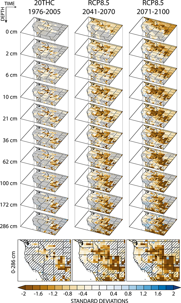
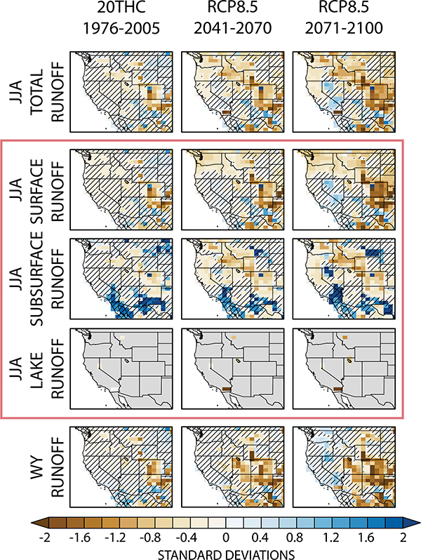
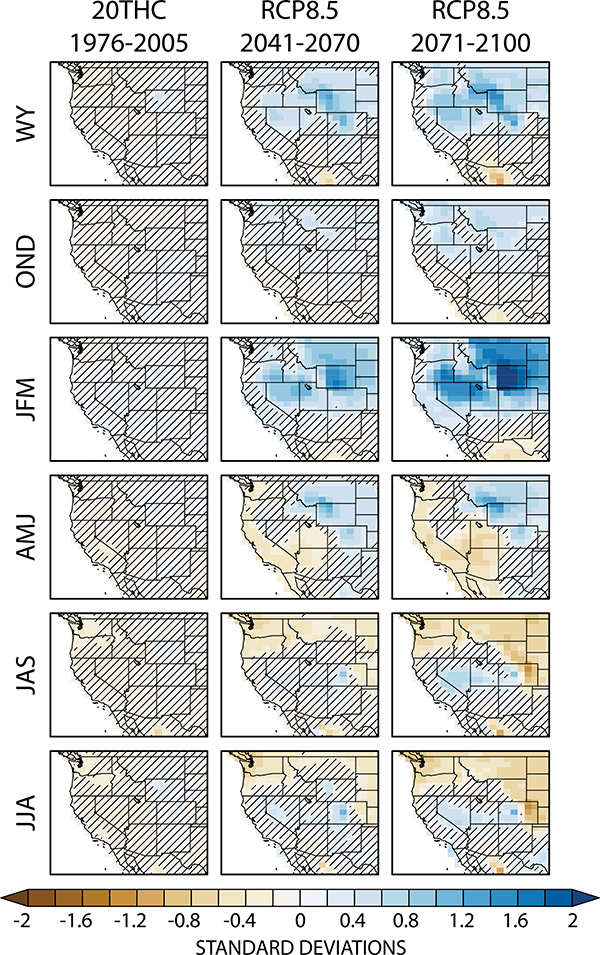
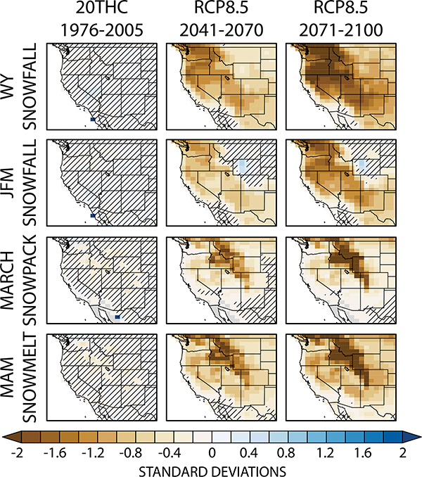
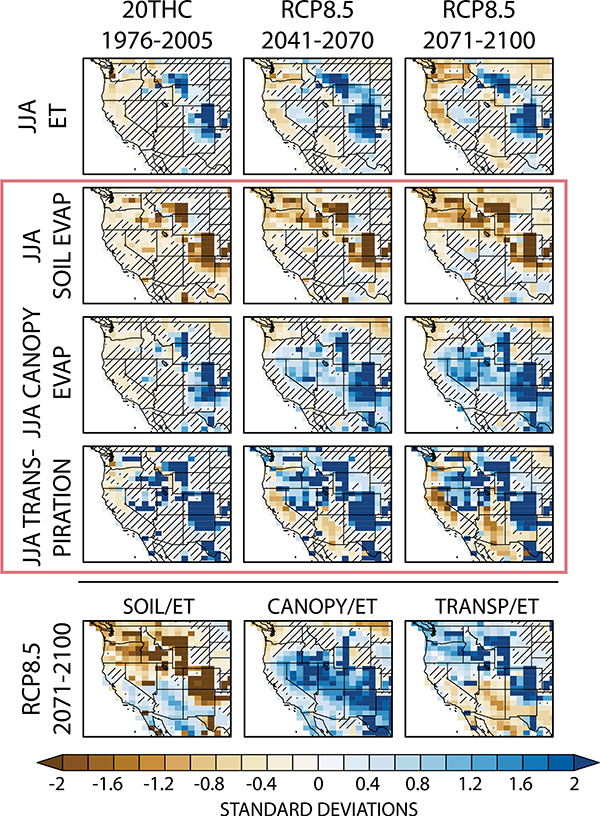
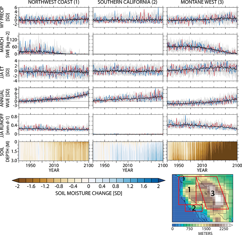
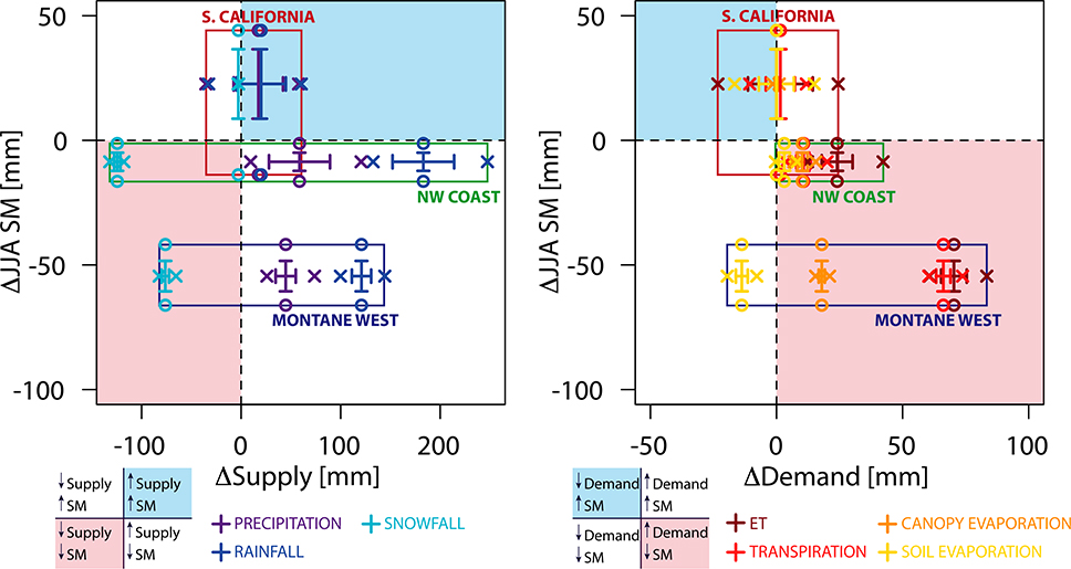
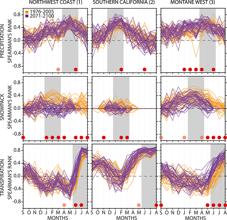
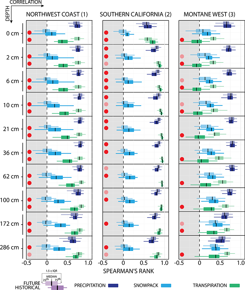
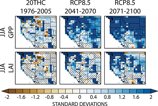
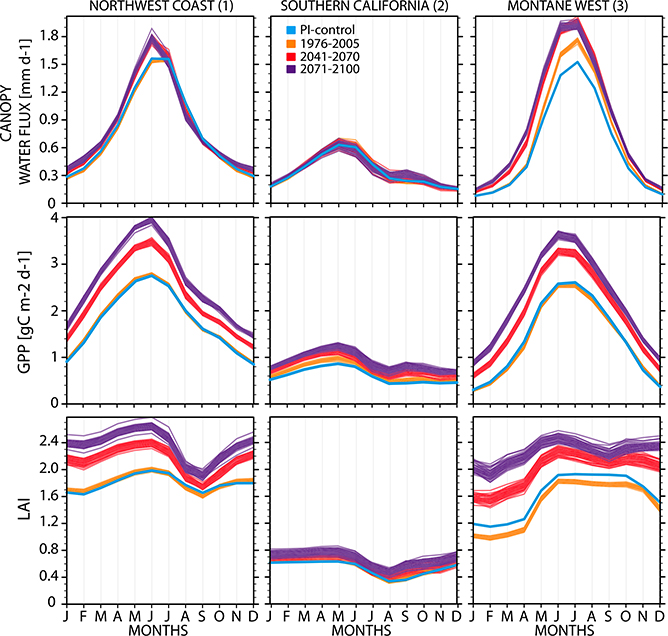
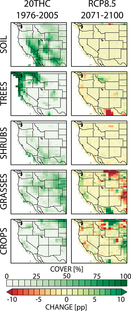
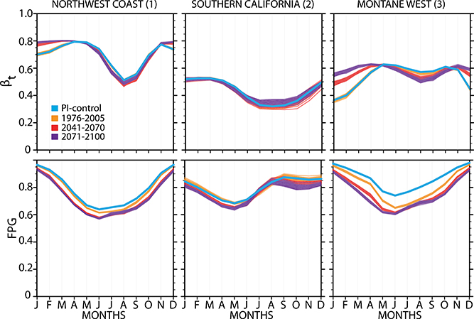
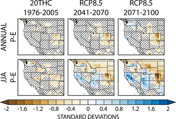
Climate models project significant twenty-first-century declines in water availability over the American West from anthropogenic warming. However, the physical mechanisms underpinning this response are poorly characterized, as are the uncertainties from vegetation's modulation of evaporative losses. To understand the drivers and uncertainties of future hydroclimate in the American West, a 35-member single model ensemble is used to examine the response of summer soil moisture and runoff to anthropogenic forcing. Widespread dry season soil moisture declines occur across the region despite increases in total water-year precipitation and ubiquitous increases in plant water-use efficiency. These modeled soil moisture declines are initially forced by significant snowpack losses that directly diminish summer soil water, even in regions where water-year precipitation increases. When snowpack priming is coupled with a warming- and CO₂-induced shift in phenology and increased primary production, widespread increases in leaf area further reduces summer soil moisture and runoff by outpacing decreased stomatal conductance from high CO₂. The net effects lead to the cooccurrence of both a "greener" and "drier" future across the western United States. Because simulated vegetation exerts a large influence on predicted changes in water availability in the American West, these findings highlight the importance of reducing the substantial uncertainties in the ecological processes increasingly incorporated into numerical Earth system models.

Fig. 1.

Summer (JJA) soil moisture response to anthropogenic forcing [(left) historical, (center) RCP8.5 midcentury, (right) RCP8.5 end of century] in (top)–(bottom) each hydrologically active layer and the full (0–~3 m) column-weighted response. Each panel shows the ensemble mean of the 30-yr average time series standardized to the 1800-yr PI-control simulation mean and standard deviation from each run. Insignificant change is denoted with hatching.

Fig. 2.

Summer (JJA) runoff response to anthropogenic forcing [(left) historical, (center) RCP8.5 mid-twenty-first century, (right) RCP8.5 end of century]. We decompose (top) JJA-mean total runoff into its three components outlined in the red box: (second row) surface, (third row) subsurface, and (fourth row) lake–glacier–wetland runoff in JJA. Water-year (WY) runoff is the bottom row. Each panel shows the ensemble mean of each run’s 30-yr average time series standardized to the 1800-yr PI-control simulation mean and standard deviation. Insignificant change is denoted with hatches.

Fig. 3.

Precipitation response to anthropogenic forcing [(left) historical, (center) RCP8.5 midcentury, and (right) RCP8.5 end-of-century]. We show (top)–(bottom) the WY (October–August), October–December (OND), JFM, AMJ, July–September (JAS), and JJA seasonal means. Each panel shows the ensemble mean of each run’s 30-yr average time series standardized to the 1800-yr PI-control simulation mean and standard deviation. Insignificant change is denoted with hatching.

Fig. 4.

Snow response to anthropogenic forcing [(left) late-twentieth century, (center) RCP8.5 midcentury, and (right) RCP8.5 end of century]. We show changes in WY and JFM snowfall, March snowpack, and MAM snowmelt. Each panel shows the ensemble mean of each run’s 30-yr average time series standardized to the 1800-yr PI-control simulation mean and standard deviation. Insignificant change is denoted with hatching.

Fig. 5.

Summertime (JJA) évapotranspiration (ET) response to anthropogenic forcing [(left) historical, (center) RCP8.5 midcentury, (right) RCP8.5 end of century]. For all panels, we show JJA seasonal means in total ET and its three components (outlined in the red box in the middle): soil evaporation, canopy evaporation, and plant transpiration. (bottom) Maps showing the end-of-century (RCP8.5, 2071–2100) change in the fraction of total JJA ET coming from each component: soil, canopy, and transpiration. Each panel shows the ensemble mean of each run’s 30-yr average time series standardized to the 1800-yr PI-control simulation mean and standard deviation. Insignificant change is denoted with hatching.

Fig. 6.

Regional time series of change, 1920–2100. For each region—(left) the Northwest Coast, (center) Southern California, and (right) the Montane West—we show the LENS time series of WY (October-August) precipitation (standardized), March snowpack (kg m⁻²), JJA evapotranspiration (ET, standardized), annual water-use efficiency (WUE, standardized), and JJA runoff (mm day⁻¹). (bottom) Contours of soil moisture as a function of depth and time. The five panels from top show the time series for each ensemble member (gray) and the ensemble mean (black). We also highlight the ensemble member with the largest Theil-Sen (T-S) linear trend estimate (red) and the smallest T-S estimate (blue). All series show change relative to the 1800-yr PI-control simulation. Inset map shows the regional domains and CESM CAM5 elevation (in m).

Fig. 7.

Summertime soil moisture budget change. For each region (the Northwest Coast, Southern California, and the Montane West), we show (left) the net end-of-century change in WY precipitation and its components, WY rainfall and snowfall, against net full-column (0–2.86 m) JJA soil moisture change and (right) the same for WY ET and its components, WY transpiration, soil evaporation, and canopy evaporation. In each, the whiskers show 1.5 × IQR (the interquartile range) of the ensemble distribution while the × and ○ symbols show the full ensemble range for supply/demand and soil moisture, respectively. Inset panels show expected changes in soil moisture based on supply/demand quadrant placements.

Fig. 8.

Monthly Spearman’s rank correlations of (top) precipitation, (middle) snowpack, and (bottom) transpiration with summer (JJA) 0–2.86-m soil moisture (except for Southern California, where we use the bottom layer, 2.86 m) for (left)–(right) the Northwest Coast, Southern California, and the Montane West. For the months preceding the JJA soil moisture (September–August), we show the ensemble range in correlations in two 30-yr time periods: historical (1976–2005, orange color) and the future (2071–2100, purple color). Months with statistically significant differences based on a bootstrapped K-S test in the ensemble distributions between historical and future are denoted with dark red dots (1% level) and light red dots (5% level) at the bottom of each panel. We also highlight in gray the months chosen for correlations presented in Fig. 9, which is based on the ensemble mean historical peak correlation.

Fig. 9.

Spearman’s rank correlation between JJA soil moisture as a function of soil level, variable, and time period (historical 1975–2005, future 2071–2100) for (left) the Northwest Coast, (center) Southern California, and (right) the Montane West. The standard box plots show the ensemble range in 30-yr correlations of area-weighted average detrended standardized time series in the selected variable with JJA soil moisture. The seasonal average used is based on the Fig. 8, which highlighted peak seasonal correlations: for the Northwest Coast and the Montane West, AMJ precipitation; for Southern California, DJF precipitation; also, for the Northwest Coast and Southern California, JFM snowpack, for the Montane West, February–April (FMA) snowpack. All regions show JJA transpiration. Dark red dots show variables with statistically significant correlation distributions at the 1% level based on a bootstrapped K-S test; light red dots show significance at the 5% level.

Fig. 10.

Vegetation response to anthropogenic forcing [(left) historical, (center) RCP8.5 midcentury, (right) RCP8.5 end of century]. We show changes in JJA (top) seasonal mean photosynthesis [gross primary productivity (GPP)] and (bottom) leaf area index (LAI). Each panel shows the ensemble mean of each run’s 30-yr average time series standardized to the 1800-yr PI-control simulation mean and standard deviation. Insignificant change is denoted with hatches.

Fig. 11.

Seasonal cycles (January-December) of (top) net canopy water flux (sum of canopy evaporation and transpiration), (middle) gross primary productivity (GPP), and (bottom) leaf area index (LAI) for each region: (left) Northwest Coast, (center) Southern California, and (right) the Montane West. For each panel, four seasonal climatologies are shown for all ensemble members, that for the PI-control in blue, the historical period (1976–2005) in orange, mid-twenty-first century (2041–70) in red, and the end of the twenty-first century (2071–2100) in purple.

Fig. 12.

Prescribed land cover changes in the LENS. We aggregate the 15 plant functional types in CLM into four vegetation classes plus soil cover (from top to bottom). The late-twentieth-century land cover grid cell percentages in each class are shown at left and the end-of-century change in that grid cell percentage, as a percentage point change (pp), at right. Note that there is no biogeography in this set of simulations; all PFTs and their changes are prescribed as boundary conditions.

Fig. 13.

Seasonal cycle of (top) the water stress parameter β_t and (bottom) the GPP nitrogen limitation down-regulation parameter FPG for PI-control (blue), 1976–2005 (orange). 2041–2070 (red), and 2071–2100 (purple).

Fig. 14.

Precipitation minus evapotranspiration (P – E): (top) at the annual scale and (bottom) for summer (JJA) [(left) historical, (center) RCP8.5 midcentury, (right) RCP8.5 end of century]. Each panel shows the ensemble mean of each run’s 30-yr average time series standardized to the 1800-yr PI-control simulation mean and standard deviation. Insignificant change is denoted with hatching.

References

1. Allen R, Pereira L, Raes D, and Smith M, 1998: Crop evapotranspiration—Guidelines for computing crop water requirements. FAO Irrigation and Drainage Paper 56, 300 pp., http://www.fao.org/docrep/X0490E/X0490E00.htm.
1. Anderegg WRL, and Coauthors, 2015: Pervasive drought legacies in forest ecosystems and their implications for carbon cycle models. Science, 349, 528–532, doi:10.1126/science.aab1833. - DOI - PubMed
1. Arora VK, and Coauthors, 2013: Carbon-concentration and carbon-climate feedbacks in CMIP5 Earth system models. J. Climate, 26, 5289–5314, doi:10.1175/JCLI-D-12-00494.1. - DOI
1. Ault TR, Cole JE, Overpeck JT, Pederson GT, and Meko DM, 2014: Assessing the risk of persistent drought using climate model simulations and paleoclimate data. J. Climate, 27, 7529–7549, doi:10.1175/JCLI-D-12-00282.1. - DOI
1. ____, Mankin JS, Cook BI, and Smerdon JE, 2016: Relative impacts of mitigation, temperature, and precipitation on 21st-century megadrought risk in the American Southwest. Sci. Adv, 2, e1600873, doi:10.1126/sciadv.1600873. - DOI - PMC - PubMed
LinkOut - more resources