Confidence Sets for Cohen's d effect size images

Abstract

Current statistical inference methods for task-fMRI suffer from two fundamental limitations. First, the focus is solely on detection of non-zero signal or signal change, a problem that is exacerbated for large scale studies (e.g. UK Biobank, N=40,000+) where the 'null hypothesis fallacy' causes even trivial effects to be determined as significant. Second, for any sample size, widely used cluster inference methods only indicate regions where a null hypothesis can be rejected, without providing any notion of spatial uncertainty about the activation. In this work, we address these issues by developing spatial Confidence Sets (CSs) on clusters found in thresholded Cohen's d effect size images. We produce an upper and lower CS to make confidence statements about brain regions where Cohen's d effect sizes have exceeded and fallen short of a non-zero threshold, respectively. The CSs convey information about the magnitude and reliability of effect sizes that is usually given separately in a t-statistic and effect estimate map. We expand the theory developed in our previous work on CSs for %BOLD change effect maps (Bowring et al., 2019) using recent results from the bootstrapping literature. By assessing the empirical coverage with 2D and 3D Monte Carlo simulations resembling fMRI data, we find our method is accurate in sample sizes as low as N=60. We compute Cohen's d CSs for the Human Connectome Project working memory task-fMRI data, illustrating the brain regions with a reliable Cohen's d response for a given threshold. By comparing the CSs with results obtained from a traditional statistical voxelwise inference, we highlight the improvement in activation localization that can be gained with the Confidence Sets.

Keywords: Cohen’s d; Confidence sets; Effect sizes; Task fmri; fMRI.

Fig. 1

Schematic of the color-coded regions we will use to visually represent the Confidence Sets (CSs) and point estimate set. The upper and lower CSs are presented in red and blue (overlapped by yellow and red) respectively. The yellow set (overlapped by red), ${\widehat{\mathcal{A}}}_c,$ is the point estimate set, the best guess from the data of voxels that have a Cohen’s $d$ effect size greater than the threshold $c=0.5$.

Fig. 2

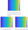
Visualizing the differences between the sample mean and sample Cohen’s $d$ field. For $N=60$ subjects, we simulated a signal-plus-noise model where the true underlying mean signal $\mu \left(\mathit{s}\right)$ was a linear ramp increasing from 0 to 10 across the region (a). To each subject we added Gaussian noise with a homogeneous variance, so that the true Cohen’s $d$ effect $d\left(\mathit{s}\right)$ was equal to the group mean signal $\mu \left(\mathit{s}\right)$. While the sample mean image $\overline{Y}\left(\mathit{s}\right)$ is uniformly smooth across the region (b), the sample Cohen’s $d$ field $\widehat{d}\left(\mathit{s}\right)$ becomes rougher from left to right (c).

Fig. 3

The two Cohen’s $d$ effects corresponding to the linear ramp signal $\mu \left(\mathit{s}\right)$. On the left, the subject-specific Gaussian noise field ${ϵ}_i\left(\mathit{s}\right)$ has a spatially constant standard deviation of 1, and therefore $d\left(\mathit{s}\right)=\mu \left(\mathit{s}\right)$. On the right, ${ϵ}_i\left(\mathit{s}\right)$ had a spatially increasing standard deviation structure in the y-direction (from top-to-bottom), while remaining constant in the x-direction.

Fig. 4

The two Cohen’s $d$ effects corresponding to the circular signal $\mu \left(\mathit{s}\right)$. On the left, the subject-specific Gaussian noise field ${ϵ}_i\left(\mathit{s}\right)$ has a spatially constant standard deviation of 1, and therefore $d\left(\mathit{s}\right)=\mu \left(\mathit{s}\right)$. On the right, ${ϵ}_i\left(\mathit{s}\right)$ had a spatially increasing standard deviation structure in the y-direction (from top-to-bottom), while remaining constant in the x-direction.

Fig. 5

Four of the Cohen’s $d$ fields $d\left(\mathit{s}\right)$ used for the 3D simulations. Plots (a)–(c) show the Cohen’s $d$ field for the three different spherical effects $\mu \left(\mathit{s}\right)$ when Gaussian noise with spatially homogeneous standard deviation was added to the signal. Plot (d) shows the Cohen’s $d$ field corresponding to the UK Biobank full mean and standard deviation images. Note that the colormap limits for the first three Cohen’s $d$ effect-size images are from 0 to 1, while the colormap limits for the UK Biobank image is from $-$0.9 to 0.9.

Fig. 6

Coverage results for the linear ramp signal, with homogeneous (top row) and heterogeneous (bottom row) Gaussian noise structures. For large sample sizes the empirical coverage performance of all three algorithms was similar, hovering slightly above the nominal level in all simulations. As the sample size was made smaller the degree of over-coverage became larger for Algorithm 1, while empirical coverage for Algorithm 2 fell below the nominal target. Algorithm 3 performed best, with all results remaining particularly close to the nominal target level for simulations using a 95% confidence level (right plots).

Fig. 7

Coverage results for the circular signal, with homogeneous (top row) and heterogeneous (bottom row) Gaussian noise structures. All algorithms performed well, and unlike the linear ramp, empirical coverage for all three methods converged towards the nominal level. For smaller sample sizes there was a larger degree of over-coverage, most noticeably for simulations using the 80% nominal target. Overall, Algorithm 2 performed marginally better than the other two methods, and Algorithm 1 performed the worst.

Fig. 8

Coverage results for the small sphere signal type, with homogeneous (top row) and heterogeneous (bottom row) Gaussian noise structures. In general, empirical coverage remained above the nominal level across all simulations, and for the 95% confidence level (right plots), the results of all three methods fell close to the nominal target (with some over-coverage for $N=30$). All methods were robust as to whether the subject-level noise had homogeneous or heterogeneous variance structure. Because of this, there are minimal differences comparing the plots between both rows.

Fig. 9

Coverage results for the large sphere signal type, with homogeneous (top row) and heterogeneous (bottom row) Gaussian noise structures. Compared with the small sphere results displayed in Fig. 9, empirical coverage results were higher for all three methods here. Algorithm 1 suffered from a particularly large degree of over-coverage for simulations with a small sample size. Coverage performance for Algorithms 2 and 3 was closer in resemblance to the corresponding small sphere results, with Algorithm 2 performing slightly better. This suggests that both of these methods are fairly robust to changes in the boundary length.

Fig. 10

Coverage results for the multiple spheres signal type, with homogeneous (top row) and heterogeneous (bottom row) Gaussian noise structures. Algorithms 2 and 3 both performed well, particularly for the 95% confidence level, where for moderate-to-large sample sizes coverage remained in the vicinity of the 95% confidence interval of the nominal target. Once again, the degree of over-coverage increased as the sample size was made smaller, most severely for Algorithm 1, while Algorithm 2 remained relatively close to the nominal level.

Fig. 11

Coverage results for the UK Biobank signal type, where the full standard deviation image was used as the standard deviation of the subject-level noise fields. Coverage results here were similar to the results for the multiple spheres signal type shown in Fig. 10. Once again, both Algorithms 2 and 3 performed well for large samples, with empirical coverage rates hovering above the nominal target, while results for Algorithm 1 came further above the nominal level. While for smaller samples the degree of over-coverage became greater for Algorithms 1 and 3, results for Algorithm 2 appear to slightly drop here.

Fig. 12

Slices views of the Cohen’s $d$ Confidence Sets obtained from applying Algorithm 3 to the HCP working memory task data, using three Cohen’s $d$ effect size thresholds, $c=0.5,0.8$ and 1.2. The upper CS ${\widehat{\mathcal{A}}}_c^{+}$ is displayed in red, and the lower CS ${\widehat{\mathcal{A}}}_c^{-}$ in blue. Yellow voxels represent the point estimate set ${\widehat{\mathcal{A}}}_c,$ the best guess from the data of voxels that have surpassed the Cohen’s $d$ threshold. The red upper CS has localized regions in the frontal gyrus, paracingulate gyrus, angular gyrus, cerebellum and precuneus which we can assert with 95% confidence have attained (at least) a 0.5 Cohen’s $d$ effect size.

Fig. 13

Comparing the upper CSs (red voxels) computed with Algorithm 3 on the HCP working memory task data (same slice views as Fig. 12) with the thresholded $t$-statistic results obtained by applying a traditional group-level one-sample $t$-test, voxelwise $p<0.05$ FWE correction (green-yellow voxels). While the thresholded statistic map contains a single cluster covering a sizable portion of the parietal lobe across both hemispheres (axial slices), the upper CSs have localized the precise areas of the precuneus and anglur gyrus where we can confidently declare a Cohen’s $d$ effect size of at least 0.5. This demonstrates how the CSs can provide improved spatial specificity in determining regions with practically significant activation.

Fig. B1

Histogram showing the distribution of effect sizes in the UK Biobank Cohen’s $d$ field used for the final 3D simulation, as shown in the bottom row of Fig. 5.

Fig. C1

Coverage results for the UK Biobank signal type simulation with a Cohen’s $d$ threshold of $c=0.5$ (instead of the $c=0.8$ threshold used for the simulation results presented in Fig. 11). For this smaller threshold, we observed valid, over-coverage for all three methods across all sample sizes, and on-the-whole the CSs performed well. In comparison to the results obtained for the larger threshold of $c=0.8$ (Fig. 11), it is notable that there is a slightly higher degree of over-coverage across all of the results here. We believe this may be in part due to inaccuracies in the interpolation method used to assess the simulations results, rather than inaccuracies in the method itself; as the boundary length $\partial {\mathcal{A}}_c$ is longer for the smaller threshold used here, it is more likely that violations of coverage were missed (due to the fact coverage is assessed at only a discrete set of lattice points along $\partial {\mathcal{A}}_c$), inducing a positive bias in the results. We discuss this issue in more depth at the end of Section 5.2.

Fig. D1

S.1:Slices views of the Cohen’s $d$ Confidence Sets obtained from applying Algorithm 1 to the HCP working memory task data, using three Cohen’s $d$ effect size thresholds, $c=0.5,0.8$ and 1.2. Comparing with Fig. 12 and Fig. D.2, the CSs presented here are slightly more conservative than the corresponding CSs obtained with Algorithms 2 and 3 (in the sense that the red upper CSs here are smaller, and blue lower CSs are larger). This is consistent with the simulation results obtained in Sections 4.1 and 4.2, where the empirical coverage for Algorithm 1 was consistently larger than the other two methods.

Fig. D2

Slices views of the Cohen’s $d$ Confidence Sets obtained from applying Algorithm 2 to the HCP working memory task data, using three Cohen’s $d$ effect size thresholds, $c=0.5,0.8$ and 1.2. Comparing with Fig. 12, the upper and lower CSs presented here are almost identical to the corresponding CSs obtained with Algorithm 3.

Fig. E1

Sensitivity results for the ramp signal, with homogeneous (top row) and heterogeneous (bottom row) Gaussian noise structures.

Fig. E2

Sensitivity results for the circular signal, with homogeneous (top row) and heterogeneous (bottom row) Gaussian noise structures.

Fig. E3

Sensitivity results for the small sphere signal, with homogeneous (top row) and heterogeneous (bottom row) Gaussian noise structures.

Fig. E4

Sensitivity results for the large sphere signal, with homogeneous (top row) and heterogeneous (bottom row) Gaussian noise structures.

Fig. E5

Sensitivity results for the multiple spheres signal, with homogeneous (top row) and heterogeneous (bottom row) Gaussian noise structures.

Fig. E6

Sensitivity results for the UK Biobank signal, where the UK Biobank full standard deviation image was used as the standard deviation of the subject-level Gaussian noise fields.

References

1. Alfaro-Almagro F., Jenkinson M., Bangerter N.K., Andersson J.L.R., Griffanti L., Douaud G., Sotiropoulos S.N., Jbabdi S., Hernandez-Fernandez M., Vallee E., Vidaurre D., Webster M., McCarthy P., Rorden C., Daducci A., Alexander D.C., Zhang H., Dragonu I., Matthews P.M., Miller K.L., Smith S.M. Image processing and quality control for the first 10,000 brain imaging datasets from UK biobank. NeuroImage. 2018;166:400–424. - PMC - PubMed
1. Bowring A., Telschow F., Schwartzman A., Nichols T.E. Spatial confidence sets for raw effect size images. NeuroImage. 2019;203:116187. doi: 10.1016/j.neuroimage.2019.116187. - DOI - PMC - PubMed
1. Button K.S., Ioannidis J.P.A., Mokrysz C., Nosek B.A., Flint J., Robinson E.S.J., Munafò M.R. Power failure: why small sample size undermines the reliability of neuroscience. Nat. Rev. Neurosci. 2013;14(5):365–376. - PubMed
1. Cacioppo J.T., Cacioppo S., Gonzaga G.C., Ogburn E.L., VanderWeele T.J. Marital satisfaction and break-ups differ across on-line and off-line meeting venues. Proc. Natl. Acad. Sci. U.S.A. 2013;110(25):10135–10140. - PMC - PubMed
1. Carp J. The secret lives of experiments: methods reporting in the fMRI literature. NeuroImage. 2012;63(1):289–300. - PubMed
Publication types