To pool or not to pool: Can we ignore cross-trial variability in FMRI?

Abstract

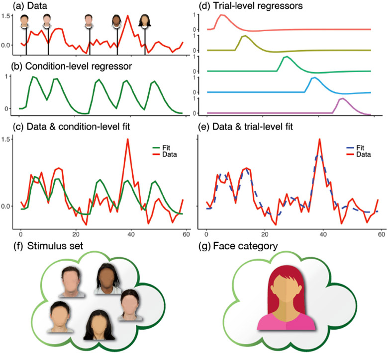
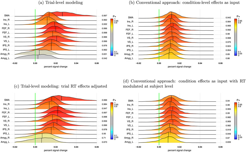
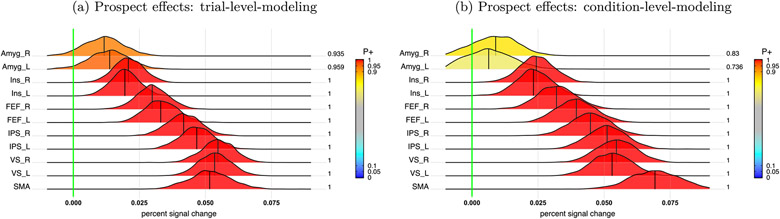
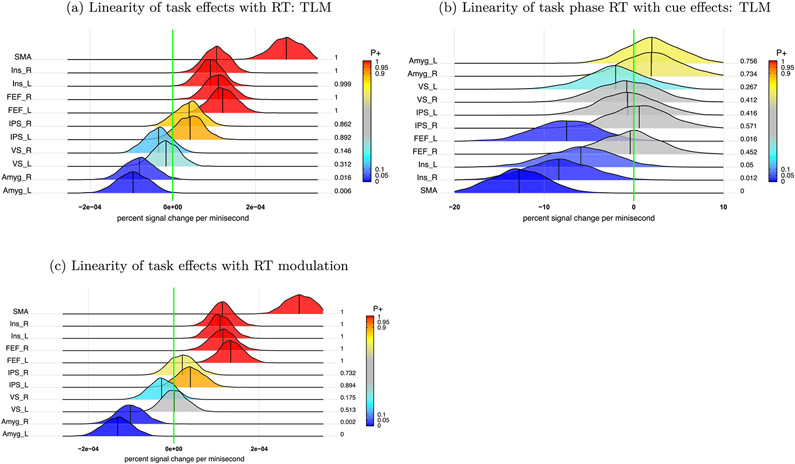
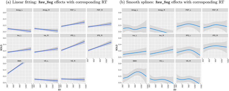
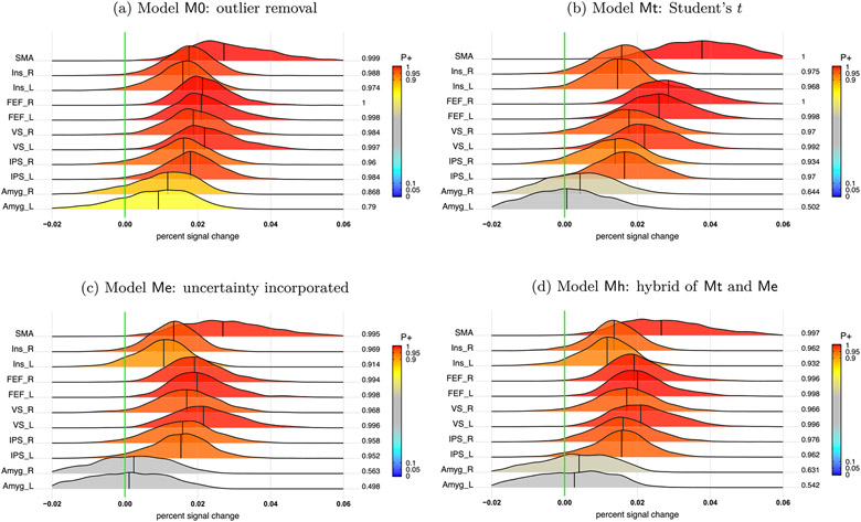
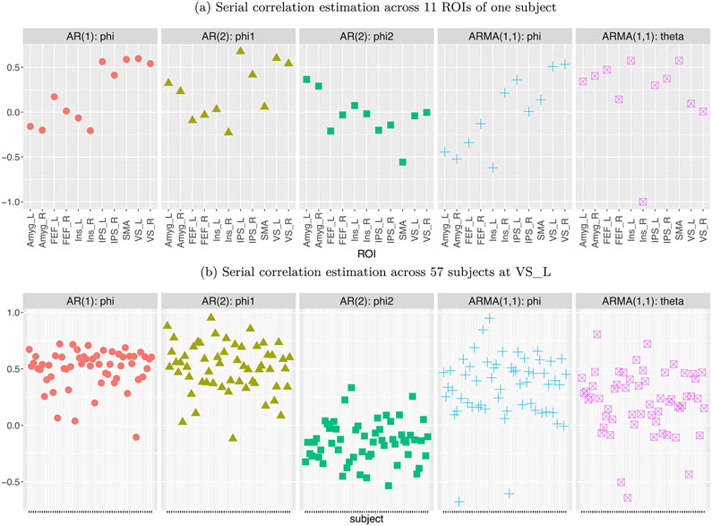
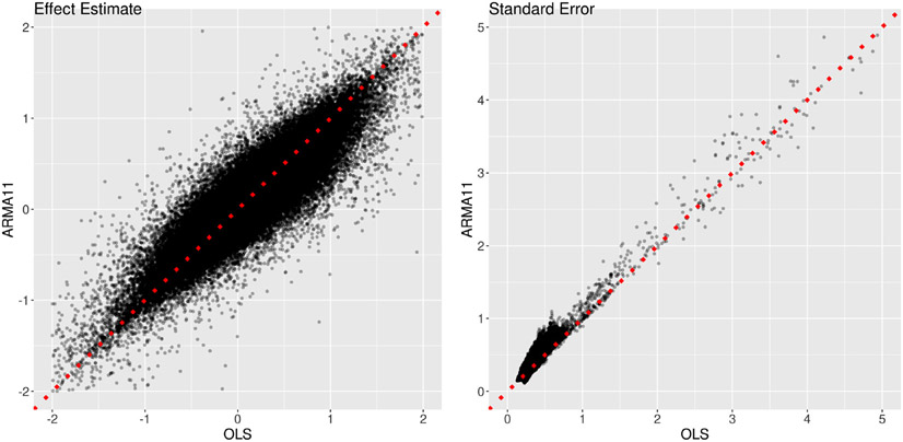
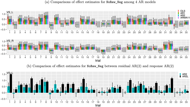
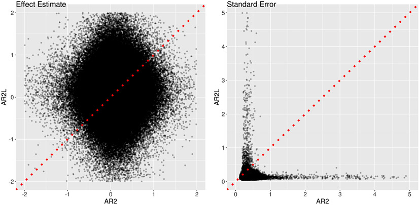
In this work, we investigate the importance of explicitly accounting for cross-trial variability in neuroimaging data analysis. To attempt to obtain reliable estimates in a task-based experiment, each condition is usually repeated across many trials. The investigator may be interested in (a) condition-level effects, (b) trial-level effects, or (c) the association of trial-level effects with the corresponding behavior data. The typical strategy for condition-level modeling is to create one regressor per condition at the subject level with the underlying assumption that responses do not change across trials. In this methodology of complete pooling, all cross-trial variability is ignored and dismissed as random noise that is swept under the rug of model residuals. Unfortunately, this framework invalidates the generalizability from the confine of specific trials (e.g., particular faces) to the associated stimulus category ("face"), and may inflate the statistical evidence when the trial sample size is not large enough. Here we propose an adaptive and computationally tractable framework that meshes well with the current two-level pipeline and explicitly accounts for trial-by-trial variability. The trial-level effects are first estimated per subject through no pooling. To allow generalizing beyond the particular stimulus set employed, the cross-trial variability is modeled at the population level through partial pooling in a multilevel model, which permits accurate effect estimation and characterization. Alternatively, trial-level estimates can be used to investigate, for example, brain-behavior associations or correlations between brain regions. Furthermore, our approach allows appropriate accounting for serial correlation, handling outliers, adapting to data skew, and capturing nonlinear brain-behavior relationships. By applying a Bayesian multilevel model framework at the level of regions of interest to an experimental dataset, we show how multiple testing can be addressed and full results reported without arbitrary dichotomization. Our approach revealed important differences compared to the conventional method at the condition level, including how the latter can distort effect magnitude and precision. Notably, in some cases our approach led to increased statistical sensitivity. In summary, our proposed framework provides an effective strategy to capture trial-by-trial responses that should be of interest to a wide community of experimentalists.

Fig. 1.

Time series modeling in neuroimaging. Consider an experiment with five face stimuli. (a) Hypothetical times series (scaled by mean value) is shown at a brain region associated with five stimuli. (b) The conventional modeling approach assumes that all stimuli produce the same response with one regressor. (c) An effect estimate (in percent signal change or scaling factor for the regressor (b)) is associated with the fit (green) at the condition level. (d) An alternative approach models each stimulus separately with one regressor per stimulus. (e) Trial-level modeling provides an improved fit (dashed blue). (f) The set of five stimuli (specific faces, blurred for privacy only) serves as a representation of and potential generalization to a condition category (face). (g) As described in the paper, trial-level estimates can be integrated via partial pooling such that inferences can be made at the general category level.

Fig. 2.

Summary of accuracy based on the BML model (8). (a) Response accuracy and the associated 95% quantile interval (color-shaded) were estimated for each of the 4 tasks. (b) Among the posterior distributions of accuracy, the bottom two rows are the main effects while the top five rows show the interactions. At the right side of each distribution lists the posterior probability of each effect being positive, P+ (area under the curve to the right of the green line that indicates zero effect), also color-coded in the distribution shading. The vertical black line under each distribution is the median (or 50% quantile). Each distribution is a kernel density estimate which smooths the posterior samples. This figure corresponds to Fig. 3B in Padmala et al. (2017).

Fig. 3.

Summary of RT data based on the BML model (9) with t-distribution. (a) The histogram of RT among correct response trials shows the aggregated information across the trials (within [28, 47]), 4 tasks and 57 subjects (bin width: 30 ms). (b) RT and the associated 95% quantile intervals were shown for each of the 4 tasks with an overall mean of 689.3ms and s.d. of 8.8ms. (c) Among the RT posterior distributions based on the trial-level model (9), the bottom two rows are the main effects while the top five rows show the the interactions. At the right side of each distribution lists the posterior probability of each effect being positive, P+ (area under the curve to the right of the green line indicating zero effect), also color-coded in the distribution shading. The black vertical segment under each distribution shows the median. (d) The counterpart result of (c) based on the condition-level RT effects aggregated cross trials (corresponding to Fig. 3A in Padmala et al. (2017)).

Fig. 4.

Synchronization among brain regions. The effect estimates (dots) with their standard errors (line segments) were obtained through the GLS model with ARMA(1,1). Some extent of synchrony existed across trials between the left and right amygdalas of a subject under two different tasks of NoRew_Neg (upper panel) and Rew_Neg (lower panel).

Fig. 5.

Distribution of the effect estimates from the GLS model with ARMA(1,1). With 11 ROIs and 57 subjects, there were $11\times {\sum }_{s=1}^{57}{\sum }_{i=1}^2{\sum }_{j=1}^2{T}_{ijs}=98461$ trial-level effect estimates (28 ≤ T_ijs ≤ 47) among the 4 tasks. A small portion (450, 0.42%) were outlying values beyond the range of [−2, 2] with the most extremes reaching −70000 and 23900. To effectively accommodate outliers, the x-axis was shrunk beyond (1, 1).

Fig. 6.

Interaction (NoRew - Rew):(Neg - Neu) at the population level. The value at the right end of each posterior distribution indicates the posterior probability of the effect being great than 0 (vertical green line), color-coded in the area under each posterior density. Four approaches were adopted to capture the interaction effect: (a) trial-level modeling through the BML model (11); (b) conventional approach: condition-level effects from each subject were fitted in the model (12); (c) covariate modeling: trial-level effects were modeled with RT as a covariate at the population level in the BML model (15); (d) conventional approach: condition-level effects with trial-level RT adjusted from each subject were fitted in the BML model (12).

Fig. 7.

Prospect effect (Rew - NoRew) during cue phase at the population level. Even though the two approaches of trial- and condition-level modeling agreed with each other to some extent in terms of statistical evidence for the contrast between Rew and NoRew, trial-level modeling (a) showed stronger evidence for both left and right amygdala than its condition-level counterpart (b).

Fig. 8.

Linear associations of task and cue effects with task phase RT at the population level. (a) Linear association of trial-level effects during the task phase with RT was assessed in the model (15). (b) Linear association of RT during the task phase with the trial-level effects during the cue phase was assessed in the model (16). (c) RT modulation effect during the task phase from the subject level was evaluated in the model (12).

Fig. 9.

Comparisons of association analysis under the task Rew_Neg between linear fitting and smoothing splines. For better visualization on the dependence of trial-level effects on RT, the trends are shown with their 95% uncertainty bands. (a) Linear fitting was assessed in the model (17). (b) Association analysis was evaluated through smoothing splines in the model (18).

Fig. 10.

Interaction (NoRew - Rew):(Neg - Neu) at the population level through four different BML versions. The value at the right end of each line indicates the posterior probability of the effect being great than 0 (vertical green line), color-coded in the area under each posterior density. Four BML models were adopted to handle outliers: (a) M0: brute force removal of values outside [−2, 2]; (b) Me: incorporation of uncertainty for effect estimates; (c) Mt: adoption of t-distribution to accommodate outliers and skewness; and (d) Mh: hybrid of Me and Mt with both the uncertainty of effect estimates and t-distribution.

Fig. 11.

Variations of temporal correlation in the residuals of subject-level time series regression across regions and subjects. The overall average first-order AR parameter of trial-level modeling across all the 11 ROIs and 57 subjects was 0.50 ±0.20,0.47 ±0.28 and 0.33 ±0.38 for AR(1), AR(2) and ARMA(1,1), respectively; the second-order parameter for AR(2) and moving average parameter for ARMA(1,1) were −0.13 ∓ −0.17 and 0.18 ±0.34, respectively. The relative magnitude of these AR parameters indicated that the first AR parameter captured substantially large proportion of the serial correlation while the second parameter in AR(2) and ARMA(1,1) remained helpful.

Fig. 12.

Comparisons of OLS and ARMA(1,1) in effect estimate and uncertainty. The effect estimates (left) and their standard errors (right) are shown for total $2\times 11\times {\sum }_{s=1}^{57}{\sum }_{i=1}^2{\sum }_{j=1}^2{T}_{ijs}=200640$ trial-level effects among the two cues and four tasks. The theoretical unbiasedness of OLS estimates can be verified by the roughly equal number of data points on the two sides of the diagonal line (dotted red). However, the instability of OLS estimation is shown by the fat cloud surrounding the diagonal line: slightly overestimation (or underestimation) of OLS was shown by 52.7% (or 45.5%) of data points above (or below) the x-axis. The precision inflation of OLS can be assessed by the proportion of data points (97.5%) above the dotted red line.

Fig. 13.

Trial-level effects under the task NoRew_Neg from one subject. (a) Effect estimates are shown at two contralateral regions, left (upper row) and right (lower row) ventral striatum. Black segments indicate one standard error, and the colors code the four different AR models (OLS, AR(1), AR(2) and ARMA(1,1)) for the residuals in the GLS model (1). Only 35 trials (out of 48) were successfully completed by the subject. Despite substantial amount of cross-trial variability, some consistent extent of synchronization was revealed across all the four models and all the five contralateral region pairs (only one pair, ventral striatum, shown here). (b) Effect estimates (AR2L, black) at left ventral striatum were obtained with AR effects modeled as second-order lagged effects of the EPI time series in the model (21) as implemented in Westfall et al. (2017). The same AR(2) results from (a) are shown (AR2, iris blue) as a comparison. The impact of incorporating lagged effects in the model was quite evident with both effect estimates and their precision substantially higher at some trials.

Fig. 14.

Comparisons of two approaches in AR handling. Two models were adopted to fit the data at the 11 ROIs, one (x-axis: AR2) with the GLS model (1)plus an AR(2) structure and the other (y-axis: AR2L) with the model (21)that mimicked the approach by Westfall et al. (2017). The effect estimates (left) and their standard errors (right) are shown for the total $2\times 11\times {\sum }_{s=1}^{57}{\sum }_{i=1}^2{\sum }_{j=1}^2{T}_{ijs}=200640$ trial-level effects among the two cues and four tasks. The substantial amount of deviation of the effect estimates from the diagonal line (dotted red) indicates the dramatic differences between the two models. The precision underestimation of the model with lagged effects (AR2L) can be assessed by the proportion of data points (98.3%) below the dotted red line.

References

1. Achen CH, 2001. Why lagged dependent variables can suppress the explanatory power of other independent variables Annual Meeting of the Political Methodology Section of the American Political Science Association. UCLA; July 20–22, 2000.
1. Baayen H, Davidson DJ, Bates DM, 2008. Mixed-effects modeling with crossed random effects for subjects and WES. J. Memory Lang. 59 (4), 390–412.
1. Bellemare MF, Masaki T, Pepinsky TB, 2017. Lagged explanatory variables and the estimation of causal effect. J. Polit 79 (3), 949–963.
1. Bullmore E, Brammer M, Williams SC, Rabe-Hesketh S, Janot N, David A, Mellers J, Howard R, Sham P, 1996. Statistical methods of estimation and inference for functional MR image analysis. Magn. Reson. Med 35, 261–277. - PubMed
1. Bürkner PC, 2018. Advanced Bayesian multilevel modeling with the r package BRMS. R J. 10 (1), 395–411.
Publication types