. 2020 Nov 12;11(1):5721.
doi: 10.1038/s41467-020-19550-x.

Laser scanning reflection-matrix microscopy for aberration-free imaging through intact mouse skull

Affiliations

Laser scanning reflection-matrix microscopy for aberration-free imaging through intact mouse skull

Seokchan Yoon et al. Nat Commun. .

Abstract

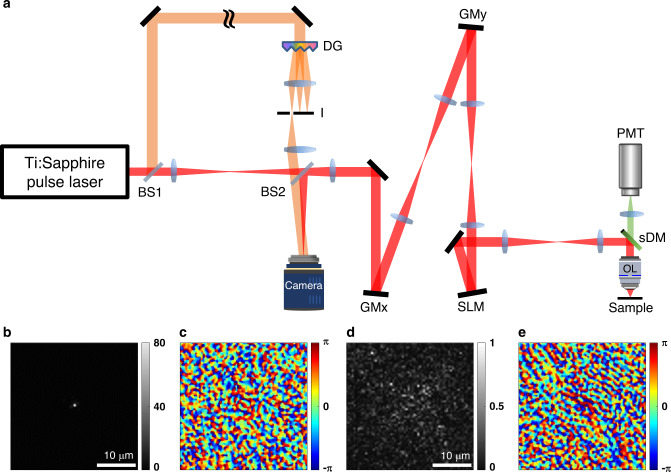
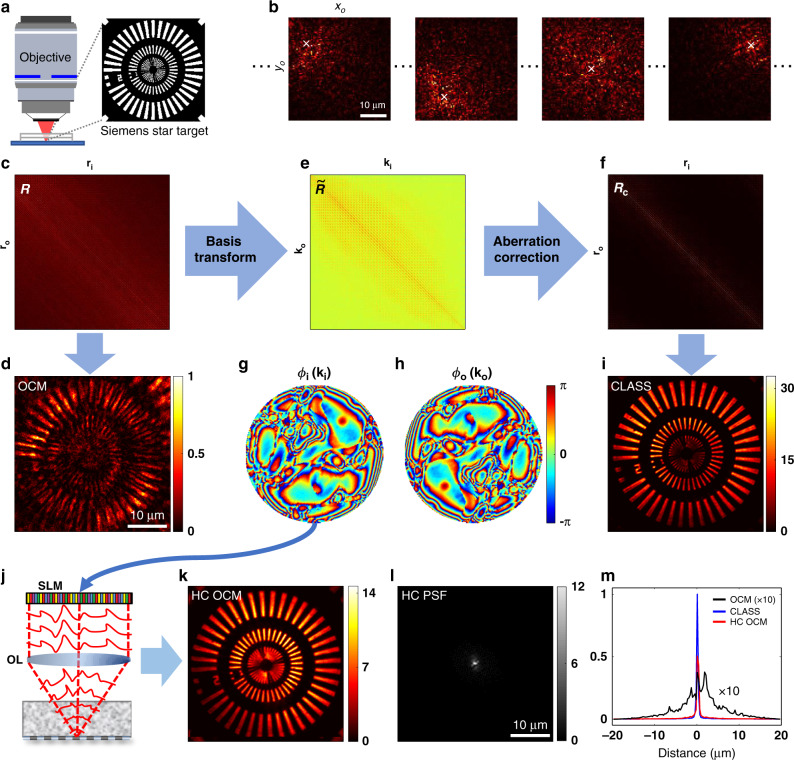
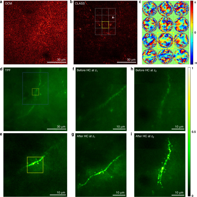
A mouse skull is a barrier for high-resolution optical imaging because its thick and inhomogeneous internal structures induce complex aberrations varying drastically from position to position. Invasive procedures creating either thinned-skull or open-skull windows are often required for the microscopic imaging of brain tissues underneath. Here, we propose a label-free imaging modality termed laser scanning reflection-matrix microscopy for recording the amplitude and phase maps of reflected waves at non-confocal points as well as confocal points. The proposed method enables us to find and computationally correct up to 10,000 angular modes of aberrations varying at every 10 × 10 µm2 patch in the sample plane. We realized reflectance imaging of myelinated axons in vivo underneath an intact mouse skull, with an ideal diffraction-limited spatial resolution of 450 nm. Furthermore, we demonstrated through-skull two-photon fluorescence imaging of neuronal dendrites and their spines by physically correcting the aberrations identified from the reflection matrix.


Conflict of interest statement

The authors declare no competing interests.

Figures

Fig. 1
Fig. 1. Experimental schematic of laser-scanning reflection-matrix microscopy.
a Experimental schematic; BS1 and BS2 beam splitters. The sample and reference beams are colored in red and orange, respectively, for visibility. GMx and GMy, galvanometer mirrors for scanning the sample beam along x and y axes, respectively. SLM spatial light modulator, sDM short-pass dichroic mirror, OL objective lens, PMT photomultiplier tube, DG diffraction grating, P pinhole. b, c Intensity and phase images of the reflected wave Ecam(rcam; ri), from the sample, respectively, for samples without aberrations. d, e Same as b and c, but for an aberrating sample. Color bars in b and d indicate intensity normalized by the maximum intensity in d. Color bars in c and e indicate phase in radians. Scale bars, 10 µm.
Fig. 2
Fig. 2. Aberration correction by the time-resolved reflection matrix.
a Sample geometry; a custom-made Siemens star target was placed under a 600-µm-thick, rough-surfaced plastic layer exhibiting strong aberrations. b Set of E-field images of reflected waves Elab(ro; ri) in the laboratory coordinates ro = (xo, yo). Four representative amplitude images are shown. The white “ × ” marks indicate illumination points ri. The FOD defined by the image size was set to 40 × 40 µm2. Scale bar, 10 µm. c Time-resolved reflection matrix R(ro; ri) in the position space constructed from the set of E-field images in b. Each image was converted to a column vector and assigned to its corresponding column in R. d OCM intensity image constructed from the main diagonal of R in c before aberration correction. Scale bar, 10 µm. e Reflection matrix R~ in spatial frequency space. f Aberration-corrected reflection matrix Rc converted from R~ after application of CLASS algorithm. g, h Phase maps ϕi(ki) and ϕo(ko) for aberrations in illumination and detection pupils retrieved by the CLASS algorithm, respectively. The radii of the maps correspond to a numerical aperture of 1.0. The number of modes Nc used for aberration correction in the pupil was about 6200. i Aberration-corrected CLASS intensity image obtained from the main diagonal of Rc in f. j Schematic of hardware wavefront correction. Conjugate of the illumination pupil phase map in g displayed on the SLM in Fig. 1a to physically compensate for the aberrations. k OCM intensity image after hardware correction (HC) of aberrations. l Intensity image of reflected PSF measured at the camera after physical aberration correction by SLM (HC PSF). Scale bar, 10 µm. m Line profiles of the PSFs obtained without wavefront correction (black), after computational wavefront correction by the CLASS algorithm (blue), and after hardware wavefront correction by SLM (red).
Fig. 3
Fig. 3. Imaging of myelinated axons through a mouse skull.
a Ex vivo specimen of a fixed mouse head. bd Ex vivo imaging of mouse brain through the thinned skull of a 7-week-old mouse. The thickness of the thinned skull was approximately 40 µm. b Conventional OCM amplitude image of myelinated fibers in the first cortex layer at a depth of 70 µm from the upper side of the thinned skull. c Aberration-corrected CLASS amplitude image. The CLASS algorithm was individually applied to 18 × 18 subregions to correct local aberrations, and the corrected images were stitched together. The size of each subregion is ~11 × 11 µm2, including overlap with adjacent areas. Microvessels (blue arrowheads) and myelinated axons (yellow arrowheads) are more clearly visible in the CLASS image. d Retrieved aberration maps for the detection pathway. The magnified map shows a representative aberration map. The number of correction modes Nc for each aberration map in d, set by the FOD, was about 3500. Color bar, phase in radians. eh Ex vivo imaging through intact skull of an 8-week-old mouse. The thickness of the skull was about 100 µm. e 3D reconstruction of SHG imaging of an intact mouse skull. The dashed red box indicates the depth at which CLASS imaging was performed. It was located 150 µm below the upper surface of the skull. f OCM amplitude image of myelinated fibers. Myelinated fibers are almost invisible. g, h CLASS amplitude image and corresponding aberration maps, respectively. The image was analyzed as in c and d. Nc in h was about 10,000. i Experimental setup for in vivo imaging through intact mouse skull. The thickness of the skull was 125−150 µm. j OCM intensity image of myelinated fibers at a 200-µm depth from the upper surface of the skull. k CLASS intensity image (upper) and the corresponding aberration map (lower) for a 30 × 30 µm2 area marked by the blue dotted box in j. l, m CLASS intensity images with their representative aberration maps for one of the 2 × 2 and 4 × 4 subregions, respectively. Nc used in aberration maps in km was about 3500. The skull thicknesses and imaging depths reported here are the raw axial movement of the sample stage.
Fig. 4
Fig. 4. TPF imaging through an intact mouse skull.
a Conventional OCM image under an intact mouse skull before aberration correction. The thickness of the skull was about 85 μm, and the focal plane was set to a depth z0 = 125 μm from the upper surface of the skull. b MIP of five LS-RMM images taken over a depth range of 117–133 μm with 4-μm steps. LS-RMM image for each depth was obtained by stitching aberration-corrected 15 × 15 subregions. Note that myelinated fibers appear discontinuous in the image mainly due to coarse depth steps and large inclination angles of the fibers with respect to the image plane. c Aberration maps of subregions at z0 = 125 μm indicated by the gray dotted boxes in b. The size of the subregion is 10 × 10 μm2, and each phase map contains 9880 angular modes. Color bar, phase in radians. d MIP of TPF images at the same position as a before hardware aberration correction. The MIP image was obtained for a depth range of 119–135 μm with a 1.5-μm increment. e TPF image after physical aberration correction for the subregion indicated by the yellow box in b. Yellow boxes in d and e correspond to the same yellow box area in b. f, g MIP of TPF images at the depth z1 = 113 ± 1.5 μm before and after aberration correction, respectively, for the area, indicated as a white dashed box in d. h, i Same as f and g, respectively, for the depth z2 = 122 ± 1.5 μm. Color bar, intensity normalized by the maximum intensity in i. Scale bars indicate 30 μm in a, b and d, and 10 μm in ei.

Similar articles

Cited by

References

    1. Minsky, M. Microscopy apparatus. US Patent 3013467 Vol. 3013467 5 (1957).
    1. Dunsby C, French PMW. Techniques for depth-resolved imaging through turbid media including coherence-gated imaging. J. Phys. D. Appl. Phys. 2003;36:R207–R227. doi: 10.1088/0022-3727/36/14/201. - DOI
    1. Pawley, J. Handbook of Biological Confocal Microscopy (Springer, US, 2010).
    1. Izatt JA, Swanson EA, Fujimoto JG, Hee MR, Owen GM. Optical coherence microscopy in scattering media. Opt. Lett. 2008;19:590. doi: 10.1364/OL.19.000590. - DOI - PubMed
    1. Booth MJ. Adaptive optical microscopy: the ongoing quest for a perfect image. Light Sci. Amp; Appl. 2014;3:e165. doi: 10.1038/lsa.2014.46. - DOI

Publication types

LinkOut - more resources