Phenotypic variation of transcriptomic cell types in mouse motor cortex

Abstract

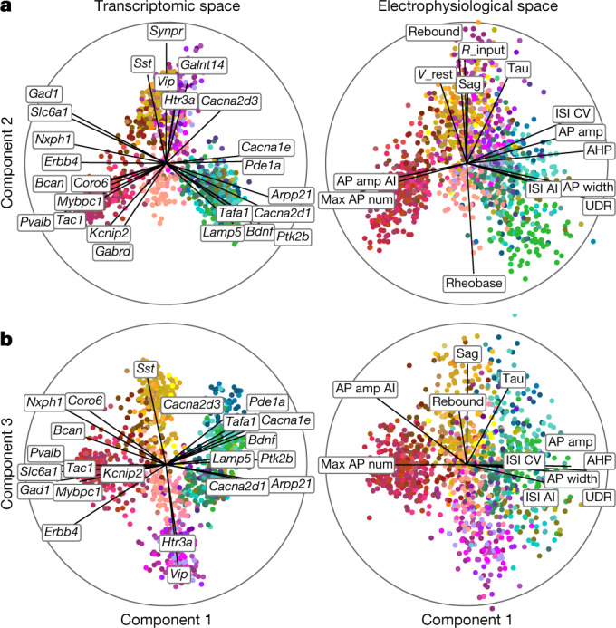
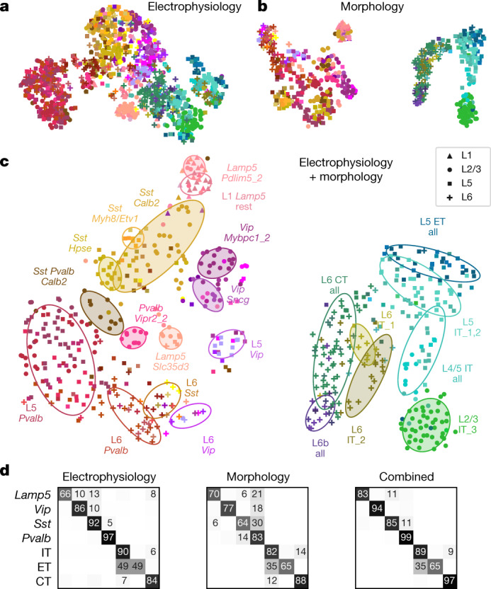
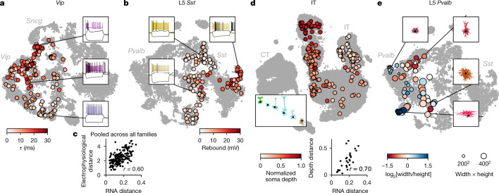
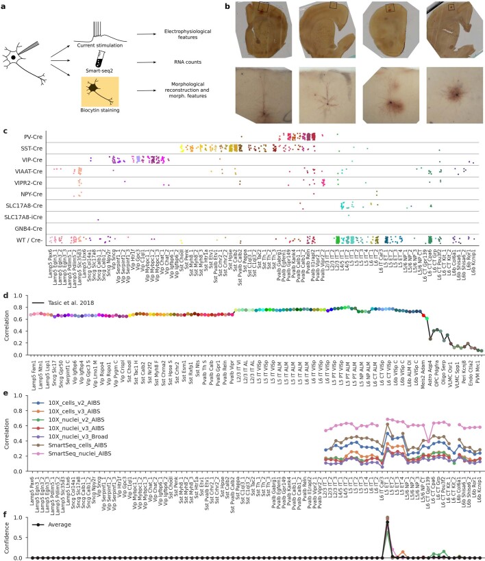
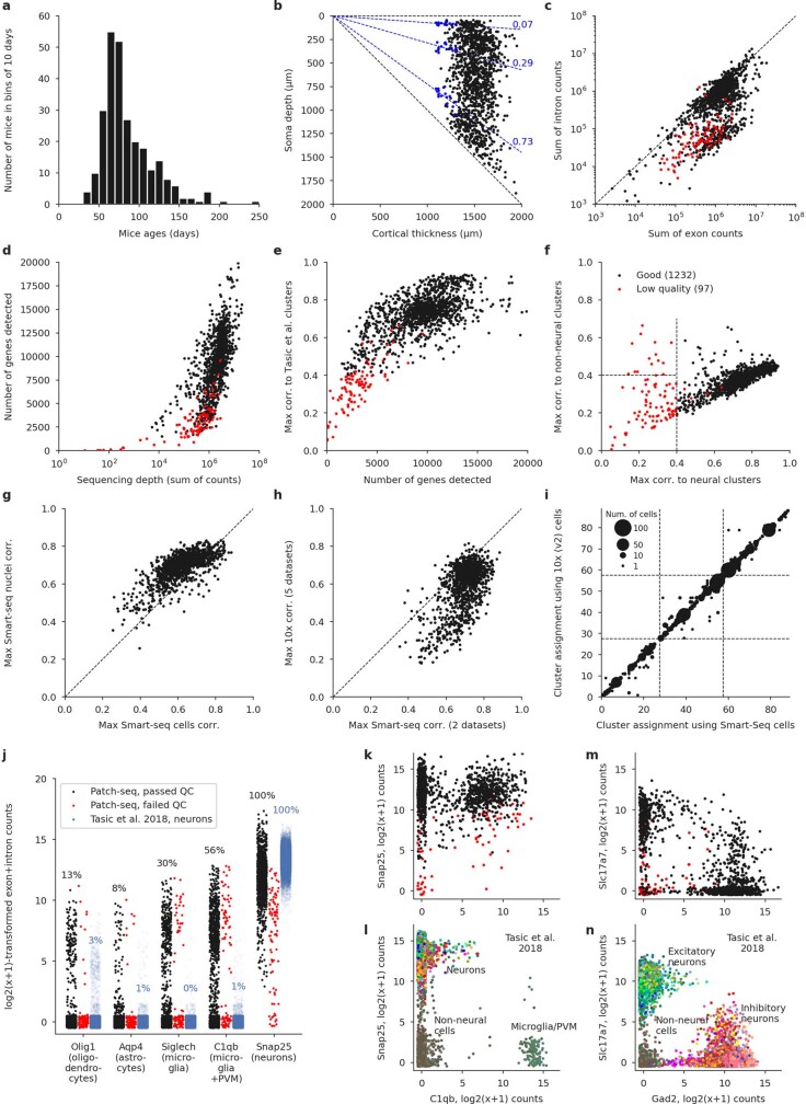
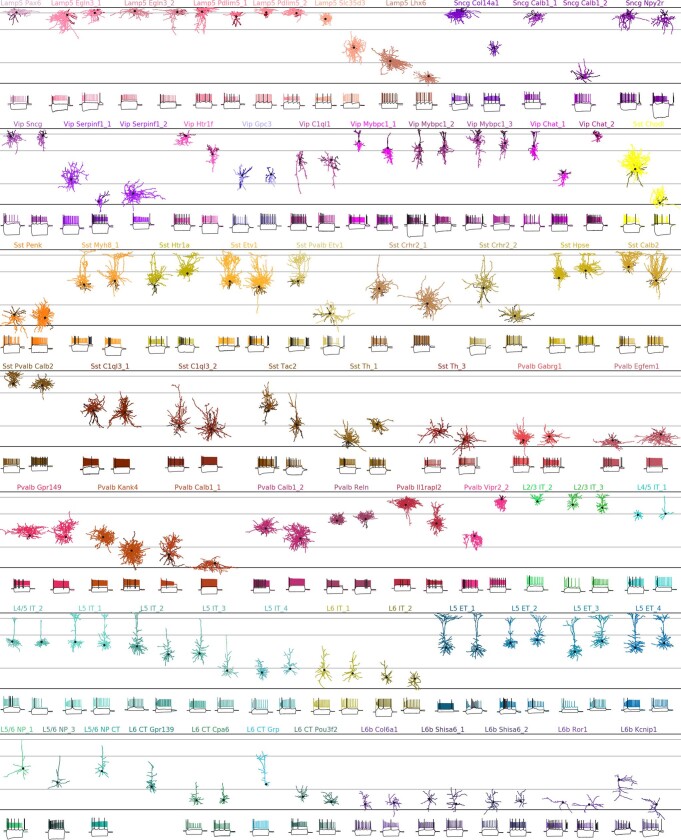
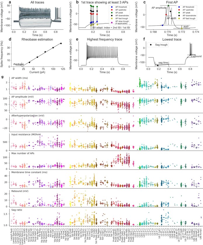
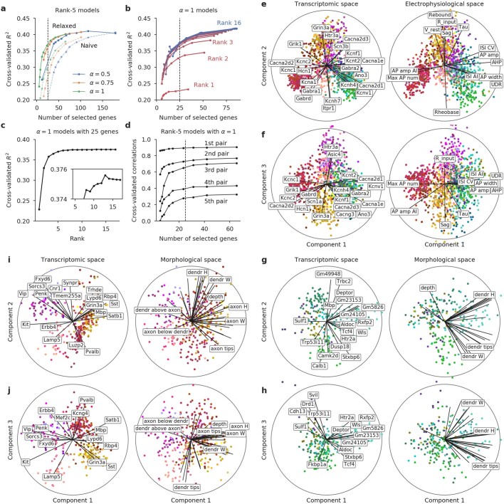
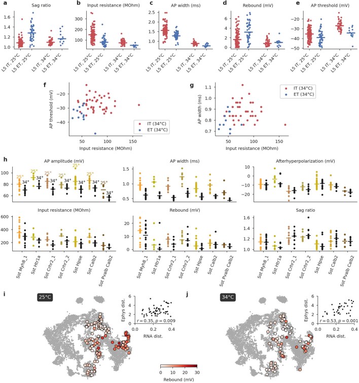
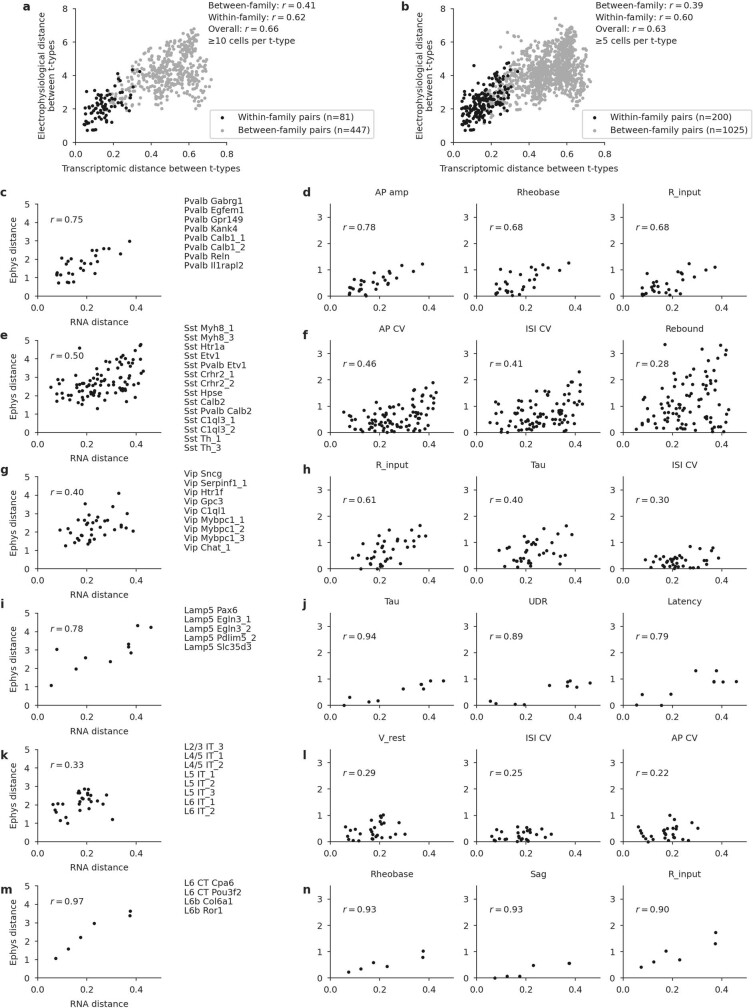
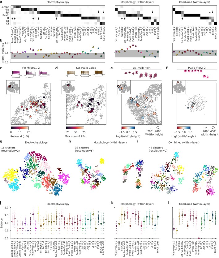
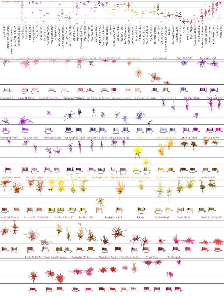
Cortical neurons exhibit extreme diversity in gene expression as well as in morphological and electrophysiological properties^1,2. Most existing neural taxonomies are based on either transcriptomic^3,4 or morpho-electric^5,6 criteria, as it has been technically challenging to study both aspects of neuronal diversity in the same set of cells⁷. Here we used Patch-seq⁸ to combine patch-clamp recording, biocytin staining, and single-cell RNA sequencing of more than 1,300 neurons in adult mouse primary motor cortex, providing a morpho-electric annotation of almost all transcriptomically defined neural cell types. We found that, although broad families of transcriptomic types (those expressing Vip, Pvalb, Sst and so on) had distinct and essentially non-overlapping morpho-electric phenotypes, individual transcriptomic types within the same family were not well separated in the morpho-electric space. Instead, there was a continuum of variability in morphology and electrophysiology, with neighbouring transcriptomic cell types showing similar morpho-electric features, often without clear boundaries between them. Our results suggest that neuronal types in the neocortex do not always form discrete entities. Instead, neurons form a hierarchy that consists of distinct non-overlapping branches at the level of families, but can form continuous and correlated transcriptomic and morpho-electrical landscapes within families.

Fig. 1. Transcriptomic coverage.

a, Number of Patch-seq cells assigned to each of the neural transcriptomic types (t-types). Colours and the order of types are taken from the original publication. The filled part of each bar shows the number of morphologically reconstructed neurons. Grey labels, t-types with no cells. Total number of neurons, 1,227. b, Normalized soma depths of all neurons of each t-type. For t-types with at least three cells, horizontal lines show medians. Soma depths were normalized by the cortical thickness in each slice (0, pia; 1, white matter). Grey horizontal lines, approximate layer boundaries identified by Nissl staining (L1, 0.07; L2/3, 0.29; L5, 0.73). Total number of neurons, 1,187 (for some cells soma depth could not be measured owing to failed staining). c, t-SNE representation of CGE-derived interneurons from the single-cell 10x v2 reference data set (n = 15,511; perplexity, 30). t-Type names are shortened by omitting the first word; some are abbreviated. Patch-seq cells from the Vip, Sncg, and Lamp5 subclasses were positioned on this t-SNE atlas (black symbols). d, As in c but for MGE-derived interneurons (n = 12,083; perplexity, 30). e, As in c but for excitatory neurons (n = 93,829; perplexity, 100). f, Example morphologies coloured by t-type. For interneurons, dendrites are shown in darker colours. For excitatory neurons, only dendrites are shown. Black dots mark soma locations. Three voltage traces are shown below for some exemplary cells: the hyperpolarization trace obtained with the smallest current stimulation, the first depolarization trace that elicited at least one action potential, and the depolarization trace showing maximal firing rate. Stimulation length, 600 ms.

Fig. 2. Sparse reduced-rank regression.

a, b, A sparse reduced-rank regression (RRR) model to predict combined electrophysiological features from gene expression. Transcriptomic data are linearly projected to a low-dimensional space that allows reconstruction of electrophysiological data; components 1 and 2 (a) and 1 and 3 (b) of rank-5 model are shown. n = 1,219. Colour corresponds to t-type. The model selected 25 genes (left). Each panel is a biplot, showing correlations of original features with both components; the circle corresponds to correlation 1. Only features with average correlation above 0.4 are shown. Labels were automatically positioned to reduce overlap. AI, adaptation index; AP, action potential; CV, coefficient of variation; ISI, interspike interval; R_input, input resistance; V_rest, resting potential; UDR, upstroke-to-downstroke ratio.

Fig. 3. Morpho-electric t-SNE embeddings.

a, t-SNE embedding constructed using electrophysiological features. Colour corresponds to t-type. n = 1,320 cells used to construct the embedding, 1,219 cells with t-type labels shown. Perplexity, 30. b, t-SNE embedding constructed using combined morphometric features and z-profiles. n = 636 cells. Perplexity, 30. c, t-SNE embedding constructed using combined electrophysiological and morphological features. n = 628 cells. Perplexity, 30. Ellipses show 80% coverage ellipses for the most prominent t-types (shaded) and for some groups of related t-types and some layer-restricted families (unshaded). We chose these groups to reduce the overlap between ellipses. d, Confusion matrices for classifying cells into seven transcriptomic families using kNN classifier (k = 10) and three feature sets. Each row shows what fraction of cells from a given family is classified in each of the seven families. The values in each row sum to 100% but only values above 5% are shown.

Fig. 4. Phenotypic variability within transcriptomic families.

a, Vip neurons mapped to the reference t-SNE embedding from Fig. 1c, coloured by membrane time constant (τ). Insets, example firing traces. b, Sst neurons from layer 5 (excluding Sst Chodl t-type) mapped to the reference t-SNE embedding from Fig. 1d, coloured by rebound value. c, Correlation between transcriptomic distances and electrophysiological distances across all 200 pairs of t-types from the same family (for 50 t-types with at least 5 cells), pooled across all families. Transcriptomic distance was computed using the reference 10x data as the correlation between average log-expression across most variable genes. Electrophysiological distance is Euclidean distance between the average feature vectors. d, IT neurons mapped to the reference t-SNE embedding from Fig. 1e, coloured by normalized soma depth. Inset, examples of IT neurons at different depths, coloured by t-type. Scatter plot used eight t-types with at least five cells and shows correlation between transcriptomic distances and cortical depth distances. Cortical depth distance is Euclidean distance between the average normalized soma depths. e, Pvalb neurons from layer 5 mapped to the reference t-SNE embedding from Fig. 1d, coloured by axonal width/height log-ratio. Circle area corresponds to the width × height product. Insets, example morphologies.

Fig. 5. Phenotypic variability of individual t-types.

a, Confusion matrix for classifying cells from each t-type into seven transcriptomic families using electrophysiological features. Only t-types with at least ten cells are shown. Values in each column sum to 1. Arrows mark t-types that are classified into wrong families more than 25% of the time. We used a kNN-based classifier with k = 10. b, Normalized total variance of features in each t-type. Higher values correspond to t-types with more variable phenotypes. Horizontal grey band, minimum to maximum normalized variances of k-means clusters. c, Three exemplary traces from Vip Mybpc1_2 cells (all with confidence ≥ 95%) and t-SNE overlay coloured by rebound. Inset, the same t-SNE embedding as in Fig. 1. Main plot, magnification. d, Three exemplary traces from Sst Pvalb Calb2 cells (confidence ≥ 95%) and t-SNE overlay coloured by maximum firing rate.

Extended Data Fig. 1. Patch-seq protocol, mouse Cre lines, and t-type assignment.

a, Patch-seq combines electrophyiological recordings, RNA sequencing using Smart-seq2, and biocytin staining in the same cell. b, Four exemplary slice images. Top: an image of the whole slice using 4x magnification. Bottom: a flattened 3D image stack using 20× magnification. From left to right: L5 ET neuron, L2/3 IT neuron, L5 Sst neuron, L5 Pvalb neuron. c, t-Types assigned to cells collected in mice from different Cre lines. ‘WT/Cre-’ stands for cells from any Cre line that were not labelled with a fluorescent indicator, or for the cells patched in wild type mice. 1,227 cells shown. d, t-Type assignment procedure for one example cell (d–f). Correlations to the mean log expression of all t-types from ref. , using 3,000 most variable genes. Maximum correlation is to the excitatory neurons. t-Type names are shortened, and every second one is omitted for compactness. e, Correlations to all excitatory t-types from ref. using all seven reference data sets and 500 most variable genes. f, t-Type assignment confidences for all seven data sets, obtained via bootstrapping over genes. The average confidence is shown in black. The mode of the average confidence was taken as the final t-type.

Extended Data Fig. 2. Quality control.

a, Age distribution of the mice used in the experiments. Median: 75 days. b, Soma depths of all cells and cortical thickness of the corresponding slices. Dashed lines show layer boundaries, based on the Nissl-stained slices (measured layer boundaries shown as blue points). All soma depths were normalized by dividing them by the cortical thickness. c, Relationship between the number of exonic and intronic counts. The apparent bimodality could be explained by whether the nucleus was extracted or not during Patch-seq aspiration. Whenever the nucleus was not extracted, low amount of nonspliced RNA led to low intronic counts; otherwise, the number of intronic and exonic counts was almost the same. Red: cells eventually failing quality control. d, Relationship between sequencing depth (total number of reads) and the number of detected genes (number of genes with non-zero counts). e, Relationship between the number of detected genes and the maximal correlation to clusters from ref. . Cells with maximal correlation below 0.4 were declared low quality. f, Relationship between the maximal correlation across neural clusters and the maximal correlation across non-neural clusters from ref. . Cells with maximal neural correlation below 0.4 were declared low quality. See Methods for additional QC criteria. g, Maximal correlations using single-cell and single-nucleus Smart-seq2 reference data sets. h, Maximal correlations using Smart-seq2 reference data sets (maximum across cell types and across two data sets) and using 10x reference data sets (maximum across cell types and across five data sets). i, t-Type assignment using single-cell Smart-seq2 reference data set and using single-cell 10x v2 reference data set. All points are on the integer grid; marker size shows the number of cells at the corresponding location. Dashed lines separate CGE-derived interneurons, MGE-derived interneurons, and excitatory neurons. The mapping was done within each order, so there cannot be any cells outside of the diagonal blocks. j, Expression of several prominent markers of non-neural cells, in comparison to the Smart-seq2 data set from ref. . The values are log₂(x + 1)-transformed sums of exonic and intronic counts, shown with random $U\left(-\frac{1}{2},\frac{1}{2}\right)$ jitter. Percentage values refer to the fraction of cells with non-zero counts. PVM stands for perivascular macrophages. We selected these markers because they have very low expression in neural cells. A neuronal marker Snap25 is shown for comparison. Cells from the reference data set are shown with the alpha-level set to the ratio of our data set size to that data set size (0.06), to make the dot plots more comparable. k, l, Neural and glial expression in our data set (k) and in the FACS-sorted data set (l) (plotted using the colours from the original publication, without transparency). m, n, The same using the excitatory marker Slc17a7 and the inhibitory marker Gad2.

Extended Data Fig. 3. Diversity of mouse cortical neurons.

Two representative examples per t-type, or one if only one reconstruction was available. In total 135 neurons in 73 t-types. For interneurons, dendrites are shown in darker colours. For excitatory neurons, only dendrites are shown. Black dots mark soma locations. Horizontal grey lines show approximate layer boundaries. Three voltage traces are shown for each neuron: the hyperpolarization trace obtained with the smallest current stimulation, the first depolarization trace eliciting at least one action potential, and the depolarization trace showing maximal firing rate. Stimulation length: 600 ms. The length of the shown voltage traces: 900 ms. Electrophysiological recording for one neuron did not pass quality control and is not shown.

Extended Data Fig. 4. Extraction and distribution of electrophysiological features.

Panels a–f show data from the same exemplary cell. a, Membrane potential responses to the consecutive step current injections. Hyperpolarizing currents were used to compute the input resistance (274.80 MOhm) and membrane time constant tau (21.95 ms). b, The first five traces showing spikes were used to compute ISI adaptation index (1.26), ISI average adaptation index (1.15), AP amplitude adaptation index (0.91) and AP amplitude average adaptation index (0.99). c, The first AP elicited in this neuron. It was used to compute AP threshold (−40.18 mV), AP amplitude (81.17 mV), AP width (0.80 ms), AHP (−12.60 mV), ADP (0 mV), UDR (1.62) and latency of the first spike (69.28 ms). d, Regression line gives the rheobase estimate (20.44 pA). e, The highest firing trace with 32 APs. This trace was used to estimate the ISI CV (0.27), ISI Fano factor (0.0014 ms), AP CV (0.17) and AP Fano factor (1.32 mV). f, The lowest hyperpolarization trace was used to compute the sag ratio (1.17), sag time (0.26 ms), sag area (31.16 mV⋅ms) and rebound (17.84 mV). g, Eight important electrophysiological features are shown for all cells across all t-types. For t-types with at least three cells, horizontal lines show median values. See Supplementary File 2 for all electrophysiological features.

Extended Data Fig. 5. Additional reduced-rank regression analysis and cross-validation.

a, Cross-validated R² of ‘naive’ and ‘relaxed’ sparse RRR solutions for various elastic net penalties (α and λ). ‘Relaxed’ means that the model was re-fit without a lasso penalty using only the selected genes; ‘naive’ means that it was not re-fit. Vertical dashed lines at 25 genes corresponds to the choice made for Fig. 2. The best performance is around ~100 genes, but we chose 25 for the sake of interpretability. The subsequent panels only show results for the ‘relaxed’ models. b, Cross-validated R² using α = 1 for different ranks from rank 1 to rank 16 (full rank). c, Cross-validated R² using α = 1 and λ needed to obtain 25 genes for different ranks. The peak performance is achieved with rank ~13 (inset), but rank-5 model used in the main text is almost as good. d, Cross-validated correlations between sequential projections of the transcriptomic and electrophysiological data sets (rank-5 models with α = 1). For any given number of selected genes, correlations decrease monotonically for higher components. e, f, Reduced-rank regression model using only ion channel genes. A full analogue of Fig. 2 but using only 328 ion channel genes (see Methods), of which 307 were detected in our data set in at least 10 cells. g–j, Reduced-rank regression model predicting morphological features. An analogue of Fig. 2 but using morphological, instead of electrophysiological features. The analysis was done separately for the excitatory (g–h) and for the inhibitory (i–j) neurons because different sets of morphological features were computed for these sets of neurons. Excitatory neurons: 269 cells, 35 features. Rank-5 model, λ = 0.59, adjusted to yield 25 genes. Only a subset of morphological features are labelled to reduce the clutter (abbreviations: “W” — width, “H” — height). Inhibitory neurons: 367 cells, 50 features, λ = 0.49.

Extended Data Fig. 6. Electrophysiological properties of IT, ET, and Sst neurons in Layer 5 at physiological temperature.

a–e, Each panel shows a comparison between L5 neurons from the IT and the ET subclasses (pooled across all t-types within each subclass). The main set of experiments was done at room temperature (25 °C). Follow-up experiments were done at physiological temperature (34 °C), in the presence of 1 mM kynurenic acid and 0.1 mM picrotoxin in order to block fast glutamatergic and GABAergic synaptic transmission. Horizontal lines show median values. The first four panels correspond to features showing the largest IT/ET differences at room temperature, according to the two-sided Wilcoxon-Mann–Whitney test statistic (and omitting several features that are very correlated with the shown ones: upstroke-to-downstroke ratio, sag time, and sag area). The last panel additionally shows one feature that showed prominent difference at 34 °C. f, g, IT and ET neurons recorded at 34 °C in two-dimensional representations using the features with highest separability. h, The change of electrophysiological properties between room temperature (25 °C) and physiological temperature (34 °C) for various t-types from the Sst subclass. Only L5 neurons are shown. Only t-types with ≥ 5 cells in both conditions are shown. Horizontal lines denote median values. AP amplitude and AP width changed the most between conditions, but the relative differences between t-types stayed roughly the same. The other four shown features did not change much, and the relative differences between t-types stayed the same. i, Overlay of the L5 Sst cells over the reference t-SNE embedding, coloured by rebound, as in Fig. 4b. The inset shows the correlation between transcriptomic distances and electrophysiological differences between all pairs of Sst t-types (only for t-types with at least 5 cells, and excluding Sst Chodl), together with its p-value. j, The same analysis as in (c) but using the experiments performed at physiological temperature. No corrections for multiple comparisons were applied.

Extended Data Fig. 7. Transcriptomic and electrophysiological distances within individual families.

a, b, Pooled within-family analysis. The same analysis as in Fig. 4c but showing within-family as well as between-family pairs of t-types. Using a cutoff of at least 10 neurons per t-type (a) and a cutoff of at least 5 neurons per t-type (b). c–n, Transcriptomic and electrophysiological distances within individual families. Only t-types with ≥ 5 neurons are used for this analysis (used t-types are listed in the second column). Transcriptomically well-isolated Sst Chodl and Pvalb Vipr2_2 were excluded. Three electrophysiological features with the highest correlation to the transcriptomic distance are shown on the right, for each family.

Extended Data Fig. 8. Phenotypic variability of individual t-types.

The extended version of Fig. 5. a, Confusion matrices for classifying cells from each t-type into seven transcriptomic families, using electrophysiological, morphological, and combined features. Only t-types with at least 10 cells are shown. For morphological and combined features we only took cells from one cortical layer. Values in each column sum to 1. Arrows mark t-types that are classified into wrong families more often than 25% of the time. We used kNN-based classifier with k = 10. b, Normalized total variance of features in each t-type. Higher values correspond to t-types with more variable phenotypes. Horizontal grey band shows the min/max normalized variances of k-means clusters. c, Three exemplary traces of cells from the Vip Mybpc1_2 type (all with confidence ≥ 95%) and t-SNE overlay coloured by the rebound. Inset: the same t-SNE embedding as in Fig. 1. Main plot: zoom-in. d, Three exemplary traces of cells from the Sst Pvalb Calb2 (confidence ≥ 95%) and t-SNE overlay coloured by the maximum firing rate. e, Exemplary morphologies of L5 cells from the Pvalb Reln type and t-SNE overlay coloured by the axonal width/height log-ratio as in Fig. 4e. f, Exemplary morphologies of Pvalb Vipr2_2 chandelier neurons and t-SNE overlay coloured by the axonal width/height log-ratio as in Fig. 4e. g–i, We used Leiden clustering to cluster the cells based on electrophysiological, morphological, and combined features. The clustering resolution was adjusted to roughly match the number of e-types, m-types, and em-types from ref. . The cluster colours in these panels are arbitrary and not the same as the colours used for t-types. j–l, For each t-type with at least 10 cells, we measured the entropy of the cluster assignments. Entropy zero corresponds to all cells getting into one cluster. Higher entropies mean that cells get distributed across many clusters. We repeated the clustering 100 times with different random seeds, and for each of them, subsampled each t-type to 10 cells to measure the entropy. Points show 100 repetitions, big markers show medians. When using morphological and combined features, all t-types were layer-restricted, as above. The t-type colours do not correspond to the colours in panels (j–i).

Extended Data Fig. 9. Interneurons assigned to the Tasic et al. t-types.

This is an exact analogue of Fig. 1b and Extended Data Fig. 3 using inhibitory t-types from ref. . It allows the direct comparison with the results from ref. . We used the same neurons as in Extended Data Fig. 3 whenever possible. 99 neurons in 55 t-types.

References

1. Harris KD, Shepherd GM. The neocortical circuit: themes and variations. Nat. Neurosci. 2015;18:170–181. doi: 10.1038/nn.3917. - DOI - PMC - PubMed
1. Tremblay R, Lee S, Rudy B. GABAergic interneurons in the neocortex: from cellular properties to circuits. Neuron. 2016;91:260–292. doi: 10.1016/j.neuron.2016.06.033. - DOI - PMC - PubMed
1. Tasic B, et al. Adult mouse cortical cell taxonomy revealed by single cell transcriptomics. Nat. Neurosci. 2016;19:335–346. doi: 10.1038/nn.4216. - DOI - PMC - PubMed
1. Tasic B, et al. Shared and distinct transcriptomic cell types across neocortical areas. Nature. 2018;563:72–78. doi: 10.1038/s41586-018-0654-5. - DOI - PMC - PubMed
1. Jiang X, et al. Principles of connectivity among morphologically defined cell types in adult neocortex. Science. 2015;350:aac9462. doi: 10.1126/science.aac9462. - DOI - PMC - PubMed
Publication types