Independent components of human brain morphology

Abstract

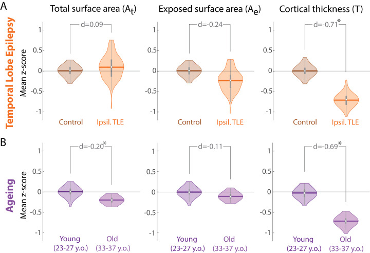
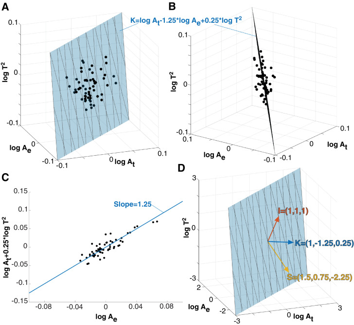
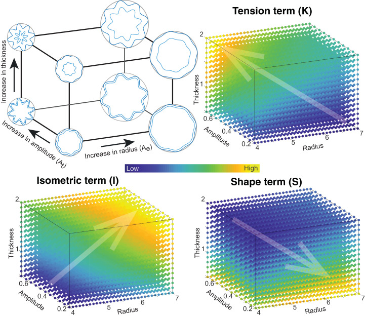
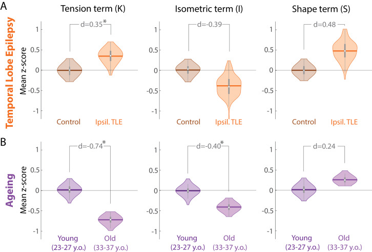
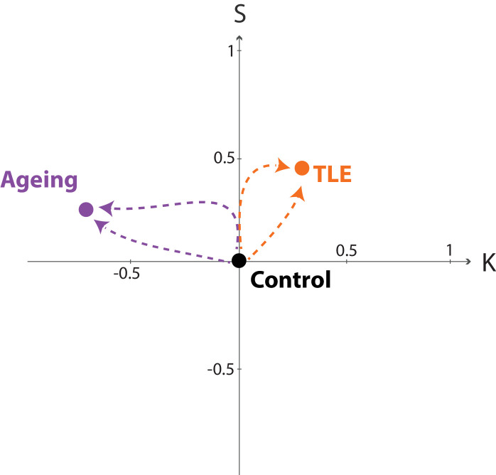
Quantification of brain morphology has become an important cornerstone in understanding brain structure. Measures of cortical morphology such as thickness and surface area are frequently used to compare groups of subjects or characterise longitudinal changes. However, such measures are often treated as independent from each other. A recently described scaling law, derived from a statistical physics model of cortical folding, demonstrates that there is a tight covariance between three commonly used cortical morphology measures: cortical thickness, total surface area, and exposed surface area. We show that assuming the independence of cortical morphology measures can hide features and potentially lead to misinterpretations. Using the scaling law, we account for the covariance between cortical morphology measures and derive novel independent measures of cortical morphology. By applying these new measures, we show that new information can be gained; in our example we show that distinct morphological alterations underlie healthy ageing compared to temporal lobe epilepsy, even on the coarse level of a whole hemisphere. We thus provide a conceptual framework for characterising cortical morphology in a statistically valid and interpretable manner, based on theoretical reasoning about the shape of the cortex.

Fig. 1

Morphology changes in TLE appear similar to those in healthy ageing. (A) Morphology changes in TLE in the ipsilateral hemisphere compared to a control cohort measured as z-scores. Violin plots show the distribution of bootstrapped mean z-scores. Age and sex correction was performed before the comparison. (B) Morphology changes in healthy ageing comparing a younger and older group of adult subjects, measured as z-scores relative to the younger subject group. Violin plots show the distribution of bootstrapped mean z-scores. Sex correction was performed before the comparison. (A & B) All morphological measures are in terms of a whole cortical hemisphere and log-scaled before analysis. Each hemisphere was treated as a separate datapoint. * denotes statistical significance at $p<0.05$. Beeswarm plots with raw data points are presented in Supplementary Data.

Fig. 2

Universal scaling law describes the covariance of the raw morphological measures. (A) Three raw morphoplogy measures span a 3D space, where each cortex is a data point (black dots). Here we used the control group in the TLE dataset as an example for the purpose of illustration. The data points align with the plane described by the universal scaling law (blue plane). (B) different viewing angle of the same data shown in (A). (C) Projection of data into a 2D space, which was previously used to visualise the scaling law. The blue line now represents the projected plane from (A) and (B). (D) 3D view of scaling law plane and viewing angle as in (A). The normal vector of the scaling law plane (K) is shown as a blue vector. Two perpendicular vectors (S and I) can be defined, and together they span the 3D space. All morphological variables are logscaled and age corrected in this figure. Cortical thickness is presented as thickness squared so that the 3D space has units of area in all dimensions.

Fig. 3

Schematic to provide intuition for the three projection terms K, S, and I Simulations of basic folded ribbons as sinusoidal oscillations on a circle. In this shape we can change the overall radius of the encapsulating circle ($A_e$), the thickness ($T$) encapsulated by the outer and inner oscillations (dark and light blue), and the amplitude of the oscillations, which dictate the total length of the oscillation ($A_t$). By scanning the radius, thickness, and oscillation amplitude in a 3D space, we can calculate the corresponding value for the $K,$$S,$ and $I$ term at different points in this space (colour map). Transparent arrows point in the directions of change of $K,$$S,$ and $I$. Through visualising the changes in $K,$$S,$ and $I$ in this 3D space, we provide an intuition for how the three terms relate to parameters in a simple folded structure.

Fig. 4

Morphological changes in K differ in TLE compared to healthy ageing. (A) Morphological changes in $K,$$S,$ and $I$ in the ipsilateral hemisphere in TLE compared to a control cohort measured as z-scores relative to controls. Violin plots show the distribution of bootstrapped mean z-scores. Age and sex correction of original morphological measures was performed before the comparison. (B) Morphological changes in healthy ageing comparing a younger and older group of adult subjects, measured as z-scores relative to the younger subject group. Violin plots show the distribution of bootstrapped mean z-scores. Sex correction of original morphological measures was performed before the comparison. (A & B) All morphological measures are in terms of a whole cortical hemisphere. Each hemisphere was treated as a separate datapoint. * denotes statistical significance at $p<0.05$. Beeswarm plots with raw data points are presented in Supplementary Data.

Fig. 5

Trajectories of morphology changes in health and disease. Visualising the changes in ageing and TLE (same data as Fig. 4) in the 2D projection into $K$ and $S$ as trajectories from the origin. We chose to show a 2D projection of $K\times S\times I$ space for simplicity. Both ageing and TLE process have been centered according to their respective control group. The respective datapoints are derived from the corresponding $d$ values in each component from Fig. 4. Dashed lines indicate possible (hypothesised) trajectories. Note that trajectories can in theory move in any direction in this space, as the axes are now independent. Shared trajectories would reflect true shared mechanisms of brain morphology change.

References

1. Alexander-Bloch A., Giedd J.N., Bullmore E. Imaging structural co-variance between human brain regions. Nat. Rev. Neurosci. 2013;14(5):322–336. doi: 10.1038/nrn3465. - DOI - PMC - PubMed
1. Aljabar P., Wolz R., Srinivasan L., Counsell S.J., Rutherford M.A., Edwards A.D., Hajnal J.V., Rueckert D. A combined manifold learning analysis of shape and appearance to characterize neonatal brain development. IEEE Trans. Med. Imaging. 2011;30(12):2072–2086. doi: 10.1109/TMI.2011.2162529. - DOI - PubMed
1. Bajaj S., Alkozei A., Dailey N.S., Killgore W.D.S. Brain aging: uncovering cortical characteristics of healthy aging in young adults. Front. Aging Neurosci. 2017;9 doi: 10.3389/fnagi.2017.00412. - DOI - PMC - PubMed
1. Bayly P.V., Taber L.A., Kroenke C.D. Mechanical forces in cerebral cortical folding: areview of measurements and models. J. Mech. Behav. Biomed.Mater. 2014;29:568–581. doi: 10.1016/j.jmbbm.2013.02.018. - DOI - PMC - PubMed
1. Carmon, J., Heege, J., Necus, J. H., Owen, T. W., Pipa, G., Kaiser, M., Taylor, P. N., Wang, Y., 2019. Reliability and comparability of human brain structural covariance networks. arXiv:1911.12755 [q-bio]ArXiv: 1911.12755. - PubMed
Publication types