Consistent population declines but idiosyncratic range shifts in Alpine orchids under global change

Abstract

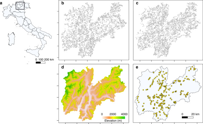
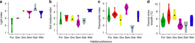
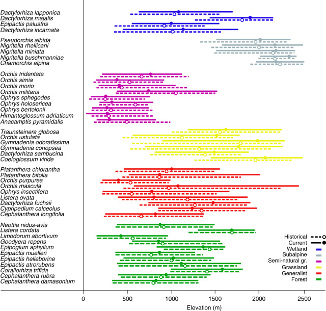
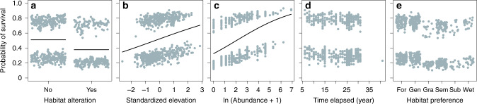
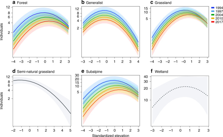
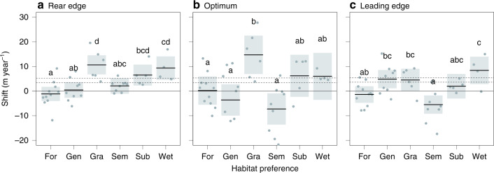
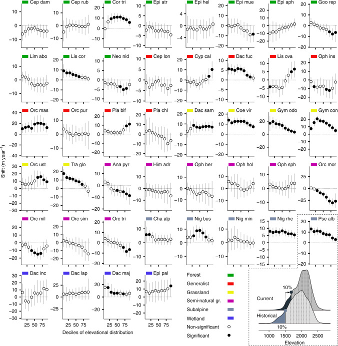
Mountains are plant biodiversity hotspots considered particularly vulnerable to multiple environmental changes. Here, we quantify population changes and range-shift dynamics along elevational gradients over the last three decades for c. two-thirds of the orchid species of the European Alps. Local extinctions were more likely for small populations, after habitat alteration, and predominated at the rear edge of species' ranges. Except for the most thermophilic species and wetland specialists, population density decreased over time. Declines were more pronounced for rear-edge populations, possibly due to multiple pressures such as climate warming, habitat alteration, and mismatched ecological interactions. Besides these demographic trends, different species exhibited idiosyncratic range shifts with more than 50% of the species lagging behind climate warming. Our study highlights the importance of long-term monitoring of populations and range distributions at fine spatial resolution to be able to fully understand the consequences of global change for orchids.

Fig. 1. Spatial location of orchid occurrence.

a Location of the study area, b geographical distribution of the sites (grey points) over the first period (1990–2003: n = 10,293) and c the second period (2004–2017: n = 11,308), d digital elevation model of the study area (resolution: 25 × 25 m) and e location of the 463 resurvey sites (yellow points).

Fig. 2. Ecological characterization of habitat preference categories.

Landolt ecological indicator values for a light (from very shady: 1 to very bright: 5), b soil moisture (from very dry: 1 to flooded: 5), c temperature (from alpine: 1 to very warm: 5) and d realized breadth of the thermal niche in the study area based on annual mean temperature. Habitat preference categories: Forest (For), Generalist (Gen), Grassland (Gra), Semi-natural grassland (Sem), Subalpine (Sub), Wetland (Wet). Violin plots were drawn using the geom_violin() function with default settings in the ggplot2 package in R. Points represent medians.

Fig. 3. Orchid elevational distribution.

Elevational distribution for the orchid species with at least 30 distribution records per period (historical, 1990–2003, and current, 2004–2017) pooled by habitat preference. Dashed bars represent historical (1990–2003) and solid bars current (2004–2017) rear (5%) and leading edges (95%), points represent optima (highest peak) of the density distribution.

Fig. 4. Biotic and abiotic drivers of local population extirpation.

Partial residual plots showing the effect of a habitat alteration, b elevation, and c population size on orchid probability of occurrence in resurveyed sites. Also non-significant effects of d time elapsed between the initial and second survey and e habitat preference were reported. Elevation was standardized to mean 0 and SD 1 to make elevational ranges comparable among species, i.e. the most negative values corresponded to the rear edge and the largest positive values to the leading edge. Plots were drawn using the visreg() function with default settings in the visreg package in R.

Fig. 5. Temporal trends in orchid population size across species elevational range.

Plots depicting the effect of time, elevation (linear and quadratic terms) and, if significant, their interaction on population size. Separate models were run for different habitat preference categories: a forest, b generalist, c grassland, d semi-natural grassland, e subalpine, and f wetland. Within each species, elevation was standardized to mean 0 and SD 1 to make elevational ranges comparable among species, i.e. the most negative values corresponded to the rear edge and the largest positive values to the leading edge. The relationship for species showing no effect of time is shown in black. For clarity reasons, colour coding shows only 5 years but orchid population size has been recorded over 28 years (1990–2017). Shading areas shows 95% confidence intervals around model estimates (solid line). For wetland (dashed line), the quadratic effect of elevation was marginal (p = 0.066, n = 534 observations for 4 species). Plots were drawn using the plotEffect() function in the effects package in R. Partial residuals were not shown due to the large number of data points.

Fig. 6. Elevation range shifts of orchids according to habitat preference.

The effect of habitat preference on range shift for a rear edge, b optimum and c leading edge. Solid lines indicate model estimates, while shaded grey areas indicate intervals of confidence (95%). Horizontal dashed lines show the expected shift to track climate change based on the current rate of warming in the study area (3.8–5.5 m year⁻¹). Forest: 11 species; generalist: 9 species; grassland: 6 species; semi-natural grassland: 9 species; subalpine: 5 species; and wetland: 4 species. Superscript letters denote significant differences (p < 0.05) in shift rates according to linear regression followed by Tukey’s post hoc test (see ‘Methods’). Plots were drawn using the visreg() function with default settings in the visreg package in R.

Fig. 7. Elevation range shift between 1990–2003 (historical) and 2004–2017 (current) along the whole elevational distribution.

For each species with >30 records per period, the shift for each decile between historical and current elevation density distribution is plotted (points). Vertical lines indicate 95% bootstrap confidence interval (CI) of each decile difference. Filled points indicate that the shift is different from 0 (p < 0.05). In the dashed outline, an example of decile comparison between the two density distributions (historical vs. current) for Pseudorchis albida (Pse alb—subalpine) is depicted: all deciles shift upwards (i.e. positive values with 95% CI not crossing the zero line) but less at the leading than at the rear edge. Abbreviations of species names: Ana pyr Anacamptis pyramidalis, Cep dam Cephalanthera damasonium, Cep lon Cephalanthera longifolia, Cep rub Cephalanthera rubra, Cha alp Chamorchis alpina, Coe vir Coeloglossum viride, Cor tri Corallorhiza trifida, Cyp cal Cypripedium calceolus, Dac fuc Dactylorhiza fuchsii, Dac inc Dactylorhiza incarnata, Dac lap Dactylorhiza lapponica, Dac maj Dactylorhiza majalis, Dac sam Dactylorhiza sambucina, Epi atr Epipactis atrorubens, Epi hel Epipactis helleborine, Epi mue Epipactis muelleri, Epi pal Epipactis palustris, Epi aph Epipogium aphyllum, Goo rep Goodyera repens, Gym con Gymnadenia conopsea, Gym odo Gymnadenia odoratissima, Him adr Himantoglossum adriaticum, Lim abo Limodorum abortivum, Lis cor Listera cordata, Lis ova Listera ovata, Neo nid Neottia nidus avis, Nig bus Nigritella buschmanniae, Nig min Nigritella miniata, Nig rhe Nigritella rhellicani, Oph ber Ophrys bertolonii, Oph hol Ophrys holosericea, Oph ins Ophrys insectifera, Oph sph Ophrys sphegodes, Orc mas Orchis mascula, Orc mil Orchis militaris, Orc mor Orchis morio, Orc pur Orchis purpurea, Orc sim Orchis simia, Orc tri Orchis tridentata, Orc ust Orchis ustulata, Pla bif Platanthera bifolia, Pla chl Platanthera chlorantha, Pse alb Pseudorchis albida, Tra glo Traunsteinera globosa.

References

1. Gottfried M, et al. Continent-wide response of mountain vegetation to climate change. Nat. Clim. Chang. 2012;2:111–115. doi: 10.1038/nclimate1329. - DOI
1. Dainese M, et al. Human disturbance and upward expansion of plants in a warming climate. Nat. Clim. Chang. 2017;7:577–580. doi: 10.1038/nclimate3337. - DOI
1. Kelly AE, Goulden ML. Rapid shifts in plant distribution with recent climate change. Proc. Natl Acad. Sci. USA. 2008;105:11823–11826. doi: 10.1073/pnas.0802891105. - DOI - PMC - PubMed
1. Lamprecht A, Semenchuk PR, Steinbauer K, Winkler M, Pauli H. Climate change leads to accelerated transformation of high-elevation vegetation in the central Alps. N. Phytol. 2018;220:447–459. doi: 10.1111/nph.15290. - DOI - PMC - PubMed
1. Bertrand R, et al. Changes in plant community composition lag behind climate warming in lowland forests. Nature. 2011;479:517–520. doi: 10.1038/nature10548. - DOI - PubMed
Publication types